Experimental Typst web edition · Veto chapter pilot

3 Micromegas X-ray Detectors for BabyIAXO

Introduction

The Micromegas detector line studied in this thesis is the low-background X-ray detection system coupled to the BabyIAXO helioscope optics. Its task is narrow but demanding: it must convert a small number of soft X rays in the $1$ – $10 keV$ region into calibrated, position-sensitive waveforms while operating at surface level, close to passive shielding, active veto panels, gas services, high-voltage channels, and data-acquisition electronics. For that reason, the detector cannot be described only as an isolated gas volume. It is a coupled instrument in which gas transport, charge amplification, readout segmentation, calibration, slow control, and veto synchronization all determine the observables used later in the background analysis.

This chapter provides the detector foundation for the rest of the thesis. It first summarizes the signal-formation physics that is needed to interpret Micromegas waveforms, then describes the microbulk Micromegas technology and the IAXO-D0/IAXO-D1 prototype implementations. The final sections connect the detector to its operating services, data-acquisition chain, and calibration procedures, leaving the detailed software implementations and large-scale background simulations to Section 4 and Section 6.

3.1 The Time Projection Chamber (TPC)

Time Projection Chambers (TPCs) are gaseous detectors in which ionization electrons drift through an electric field toward a segmented readout plane. Large TPCs are often used as tracking detectors, but the BabyIAXO Micromegas detector is a shallow X-ray TPC: the relevant information is not a long momentum-measuring trajectory, but the amount of deposited charge, its two-dimensional distribution on the readout strips, and the relative timing of the digitized pulses. This compact topology is precisely what makes the detector useful for axion searches, because focused solar X rays should produce localized charge clusters while many background events produce more extended, asymmetric, or veto-correlated signatures.

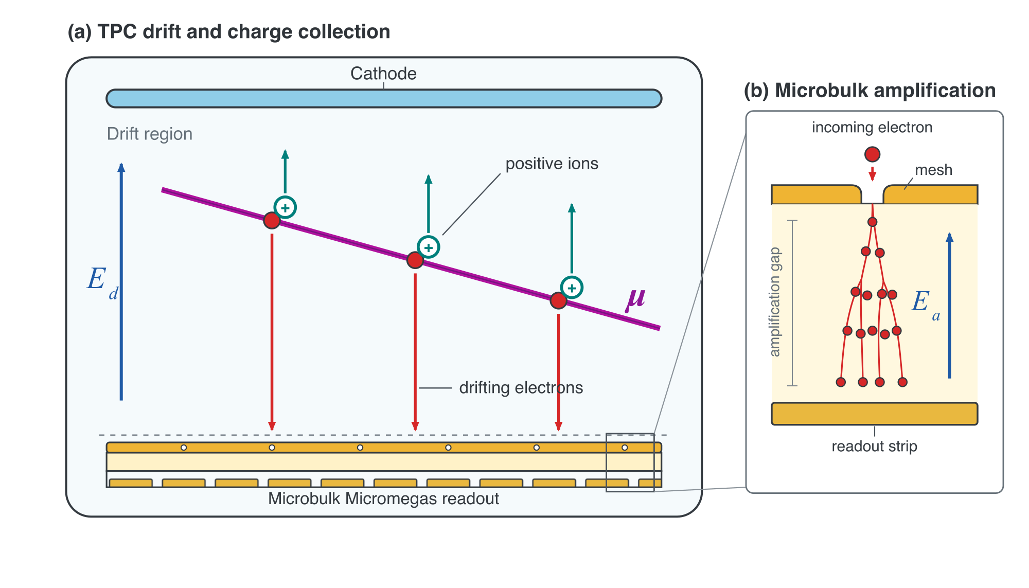
A TPC typically consists of a gas-filled chamber subjected to a uniform drift field. An incoming particle or photon interaction produces electron-ion pairs in the gas. The electrons drift toward the anode, diffuse during transport, enter an amplification region, and finally induce signals on the readout electrodes. The ions drift more slowly toward the cathode. In the BabyIAXO detector, the readout plane is a microbulk Micromegas, which combines amplification and fine strip segmentation in a radiopure structure suitable for low-background operation.

Figure 3.1: Schematic representation of a Time Projection Chamber (TPC). The ionization of the gas medium by an incoming particle results in the generation of electrons. The electrons drift toward the anode under the influence of an electric field 𝐸 𝑑 and are amplified upon reaching the amplification region where a higher electric field 𝐸 𝑎 is applied. — Figure 3.1: Schematic representation of a Time Projection Chamber (TPC). The ionization of the gas medium by an incoming particle results in the generation of electrons. The electrons drift toward the anode under the influence of an electric field $𝐸_{𝑑}$ and are amplified upon reaching the amplification region where a higher electric field $𝐸_{𝑎}$ is applied.

3.1.1 Ionization in Gases

The Micromegas signal starts with an energy deposition in the gas. For the soft X rays relevant to BabyIAXO this deposition is dominated by photoelectric absorption, whereas charged particles usually produce extended ionization tracks and neutral particles contribute indirectly through recoils or secondary radiation. Only the aspects of these processes that determine the later waveform and calibration response are summarized here.

For photons, the attenuation through a material is described by

𝐼 (𝑥) = 𝐼_{0} 𝑒^{- 𝜇 𝑥} .

(3.1)

Here, $𝜇$ is the linear attenuation coefficient. Equivalently, $𝜇 = 𝜌 𝜇_{𝑚}$ , with $𝜇_{𝑚}$ the mass attenuation coefficient. In the few-keV signal region, the photoelectric effect dominates the attenuation and produces a localized primary-electron cloud. The full background simulation transports the other electromagnetic processes, but they are not needed to explain the calibration and signal topology developed in this chapter.

Figure 3.2: Photoelectric attenuation coefficient for noble gases as a function of energy (left) and total attenuation coefficient for some saturated hydrocarbons, commonly used in gaseous mixtures as quenchers, with argon for comparison (right). Data from [ 68 ] evaluated at a temperature of 25 ∘ C and a pressure of 1 bar . — Figure 3.2: Photoelectric attenuation coefficient for noble gases as a function of energy (left) and total attenuation coefficient for some saturated hydrocarbons, commonly used in gaseous mixtures as quenchers, with argon for comparison (right). Data from [68] evaluated at a temperature of $25^{\circ} C$ and a pressure of $1 bar$ .

The preference for noble gases follows directly from the strong $𝑍$ dependence of the photoelectric cross section in the X-ray range, visible in Figure 3.2. The quencher is present at much lower concentration and has a smaller attenuation contribution, but it is essential for stable proportional operation. After photoelectric absorption, the atomic vacancy relaxes through Auger emission or fluorescence. If a fluorescent x ray escapes the sensitive volume, the measured energy is reduced and an escape feature appears in the calibration spectrum; this is particularly visible for argon-based $^{55} Fe$ calibrations.

Charged particles instead leave ionization along their path, with a topology governed by the stopping power, multiple scattering, and possible secondary radiation. In a Micromegas TPC this typically produces broader and more track-like charge patterns than a few-keV X ray. Neutral particles are relevant because they can generate nuclear recoils or secondary photons and charged particles in the gas or surrounding materials. This indirect character is one of the reasons why the background model treats radiation transport and detector-response reconstruction together rather than as separable problems.

3.1.2 Electron Transport

3.1.2.1 Primary Charge Production

An electron-recoil energy deposit $𝐸$ in the gas produces a finite number of electron-ion pairs. The electrons, referred to here as primary charge, are the carriers that drift toward the Micromegas readout and seed the avalanche in the amplification gap. The mean number of primary electrons is

𝑁_{𝑒} = \frac{𝐸}{𝑊} .

(3.2)

Here, $𝑊$ is the average energy required to create one electron-ion pair in the mixture. For nuclear recoils, part of the kinetic energy goes into atomic motion rather than ionization, so the corresponding charge yield requires a recoil-response model, discussed in Appendix Section A.1.2. The intrinsic fluctuation around this mean is smaller than Poissonian and is commonly written as

𝜎_{𝑒}^{2} = 𝐹 𝑁_{𝑒} .

(3.3)

Here, $𝐹$ is the Fano factor [69]. This primary-charge statistics sets the best achievable energy resolution before transport, amplification, and electronics effects are included.

3.1.2.2 Electron Drift

The drift field transports the primary electrons from the conversion point to the amplification region. In the mobility approximation, the drift velocity can be written as

{\vec{𝑣}}_{𝑑} = - 𝜇_{𝑒} \vec{𝐸} .

(3.4)

Here, $𝜇_{𝑒} > 0$ is the magnitude of the electron mobility at the operating field, gas density, and composition; the minus sign expresses motion opposite to $\vec{𝐸}$ . At fixed temperature, transport tables are conveniently compared using the reduced field $𝐸 / 𝑝$ , where $𝑝$ is the pressure; $𝐸 / 𝑁$ , with $𝑁$ the gas number density, is the more general variable when temperature changes. In practice, drift velocities and diffusion coefficients are taken from gas-transport calculations such as Garfield++/Magboltz, because the response depends on the mixture, pressure, field, and quencher fraction. Typical electron drift velocities in noble-gas TPC mixtures are of order $1 cm {mus}^{- 1}$ , so the drift time is directly connected to the pulse timing in the digitized waveform. The gas-mixture dependence of the drift velocity and diffusion coefficients is discussed below in the context of the detector-response gas tables.

During transport the charge cloud also diffuses. The standard deviation $𝜎_{\hat{𝑢}}$ of the electron cloud in a given direction $\hat{𝑢}$ after a drift distance $𝑑$ can be written as

𝜎_{\hat{𝑢}} = 𝐷_{\hat{𝑢}} \sqrt{𝑑} .

(3.5)

The coefficients $𝐷_{\hat{𝑢}}$ in this convention have units of square-root length, as in the Garfield++ gas [70]. They are related to the conventional diffusion coefficients ${𝒟︀}_{\hat{𝑢}}$ , with units of length squared per time, by $𝐷_{\hat{𝑢}} = \sqrt{2 {𝒟︀}_{\hat{𝑢}} / | {\vec{𝑣}}_{𝑑} |}$ for uniform drift.

Figure 3.3: Technical cutaway of electron diffusion in a TPC. Successive outlined and hatched contours show the growth of the one-standard-deviation envelope as primary charge drifts toward the Microbulk readout. In the final cloud, 𝜎 𝐿 is measured parallel to the mean drift direction and 𝜎 𝑇 perpendicular to it; both arrows extend from the centroid to the one-standard-deviation contour and therefore denote semi-axes. — Figure 3.3: Technical cutaway of electron diffusion in a TPC. Successive outlined and hatched contours show the growth of the one-standard-deviation envelope as primary charge drifts toward the Microbulk readout. In the final cloud, $𝜎_{𝐿}$ is measured parallel to the mean drift direction and $𝜎_{𝑇}$ perpendicular to it; both arrows extend from the centroid to the one-standard-deviation contour and therefore denote semi-axes.

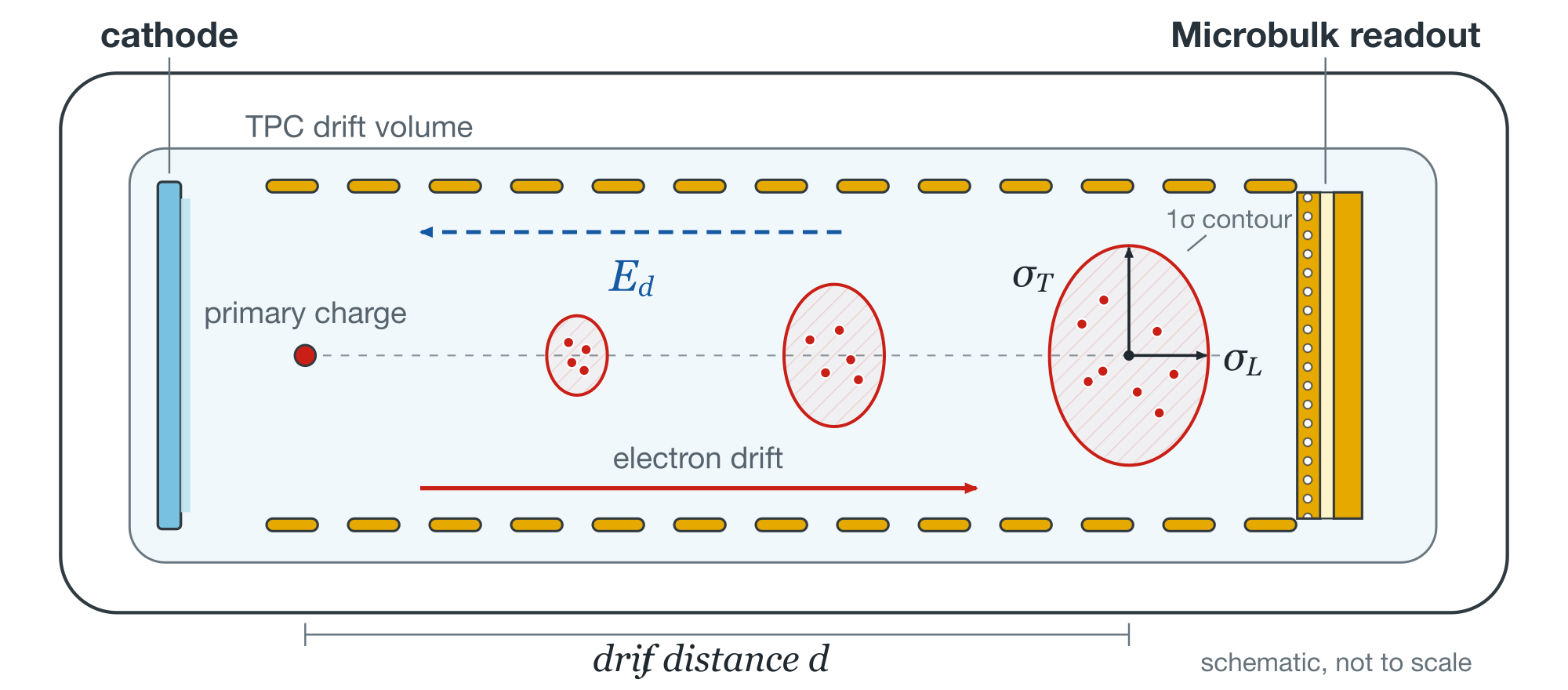
In the longitudinal section shown in Figure 3.3, the primary charge drifts opposite to the electric field. The longitudinal width $𝜎_{𝐿}$ is parallel to the mean drift direction, whereas the transverse width $𝜎_{𝑇}$ is perpendicular to it. Both are defined from the charge-cloud centroid to its one-standard-deviation contour; they are therefore semi-axes of the contour, not full cloud diameters. The separate longitudinal and transverse diffusion coefficients arise in the presence of the drift field. Diffusion controls the charge sharing between strips and the apparent width of a localized X-ray event. Recombination and attachment provide the competing loss mechanisms; in practice, oxygen and water contamination are the main operational concerns, which is why gas purity, material outgassing, and circulation are part of the detector response rather than purely auxiliary services.

3.1.2.3 Charge Amplification

The primary charge is too small to be measured directly, so the Micromegas gap operates in avalanche mode. The high amplification field converts each primary electron into a charge packet whose mean size is set by the gas gain.

The mean electron population $𝑁_{𝑎}$ after amplification of $𝑁_{𝑒}$ primary electrons across a gap of length $𝐿$ is, when attachment is negligible,

𝑁_{𝑎} = 𝑁_{𝑒} 𝑒^{\int_{0}^{𝐿} 𝛼 (𝑥) d 𝑥} .

(3.6)

Here, $𝛼$ is the first Townsend coefficient, which depends on the gas medium and the electric field. The number of electrons after amplification of the primary charge $𝑁_{𝑎}$ can be expressed as

𝑁_{𝑎} = 𝐺 𝑁_{𝑒} .

(3.7)

If the gain fluctuations of individual primary electrons are described by a variance $𝜎_{𝐺}^{2}$ , the variance of the amplified electron population, $𝜎_{𝑎}^{2}$ , can be written as

𝜎_{𝑎}^{2} = 𝐺^{2} 𝜎_{𝑒}^{2} + 𝑁_{𝑒} 𝜎_{𝐺}^{2} = 𝐺^{2} 𝑁_{𝑒} (𝐹 + 𝑏) .

(3.8)

Here, $𝑏$ is defined as

𝑏 = \frac{𝜎_{𝐺}^{2}}{𝐺^{2}} .

(3.9)

For an approximately Gaussian peak, the resolution $𝑅 = 2 \sqrt{2 ln 2} 𝜎_{𝑎} / 𝑁_{𝑎} \approx 2.35 \cdot 𝜎_{𝑎} / 𝑁_{𝑎}$ is the full width at half maximum (FWHM) of the amplified-charge distribution divided by its mean value.

𝑅 \approx 2.35 \sqrt{\frac{1}{𝑁_{𝑒}} (𝐹 + 𝑏) + {(\frac{𝜎_{el}}{𝐺 𝑁_{𝑒}})}^{2}} .

(3.10)

Here, $𝜎_{el}$ represents additional electronic-noise contributions referred to the amplified charge. The expression assumes independent single-electron avalanches and additive noise uncorrelated with the primary charge [71]. The resolution $𝑅$ is commonly expressed as a percentage.

Figure 3.4: Simplified primary-charge simulation for X rays from a 55 Fe source in a 6 cm × 6 cm × 3 cm gas volume. The photons are emitted from the center of one 6 cm × 6 cm face toward the geometric center of the volume. For the argon mixture the pressure is 1.4 bar and the drift field is 135 V cm − 1 ; for the xenon mixture they are 1.05 bar and 110 V cm − 1 , respectively. Both mixtures are evaluated at 20 ∘ C . Gaussian fits to the main primary-charge peaks give centroids of 222.29 and 205.35 electrons and absolute FWHM values of 15.05 and 14.43 electrons for argon and xenon–neon, respectively. The corresponding relative resolutions are 𝑅 = 6.77 % and 7.03 % , obtained by dividing each width by its centroid. Error bars show 68.27% Garwood intervals on the simulated bin counts, divided by the total sample size. The argon escape structure is visible at lower charge; the zero-electron population includes photons that do not produce collected primary ionization in this simplified volume. — Figure 3.4: Simplified primary-charge simulation for X rays from a $^{55} Fe$ source in a $6 cm \times 6 cm \times 3 cm$ gas volume. The photons are emitted from the center of one $6 cm \times 6 cm$ face toward the geometric center of the volume. For the argon mixture the pressure is $1.4 bar$ and the drift field is $135 V {cm}^{- 1}$ ; for the xenon mixture they are $1.05 bar$ and $110 V {cm}^{- 1}$ , respectively. Both mixtures are evaluated at $20^{\circ} C$ . Gaussian fits to the main primary-charge peaks give centroids of 222.29 and 205.35 electrons and absolute FWHM values of 15.05 and 14.43 electrons for argon and xenon–neon, respectively. The corresponding relative resolutions are $𝑅 = 6.77 %$ and $7.03 %$ , obtained by dividing each width by its centroid. Error bars show 68.27% Garwood intervals on the simulated bin counts, divided by the total sample size. The argon escape structure is visible at lower charge; the zero-electron population includes photons that do not produce collected primary ionization in this simplified volume.

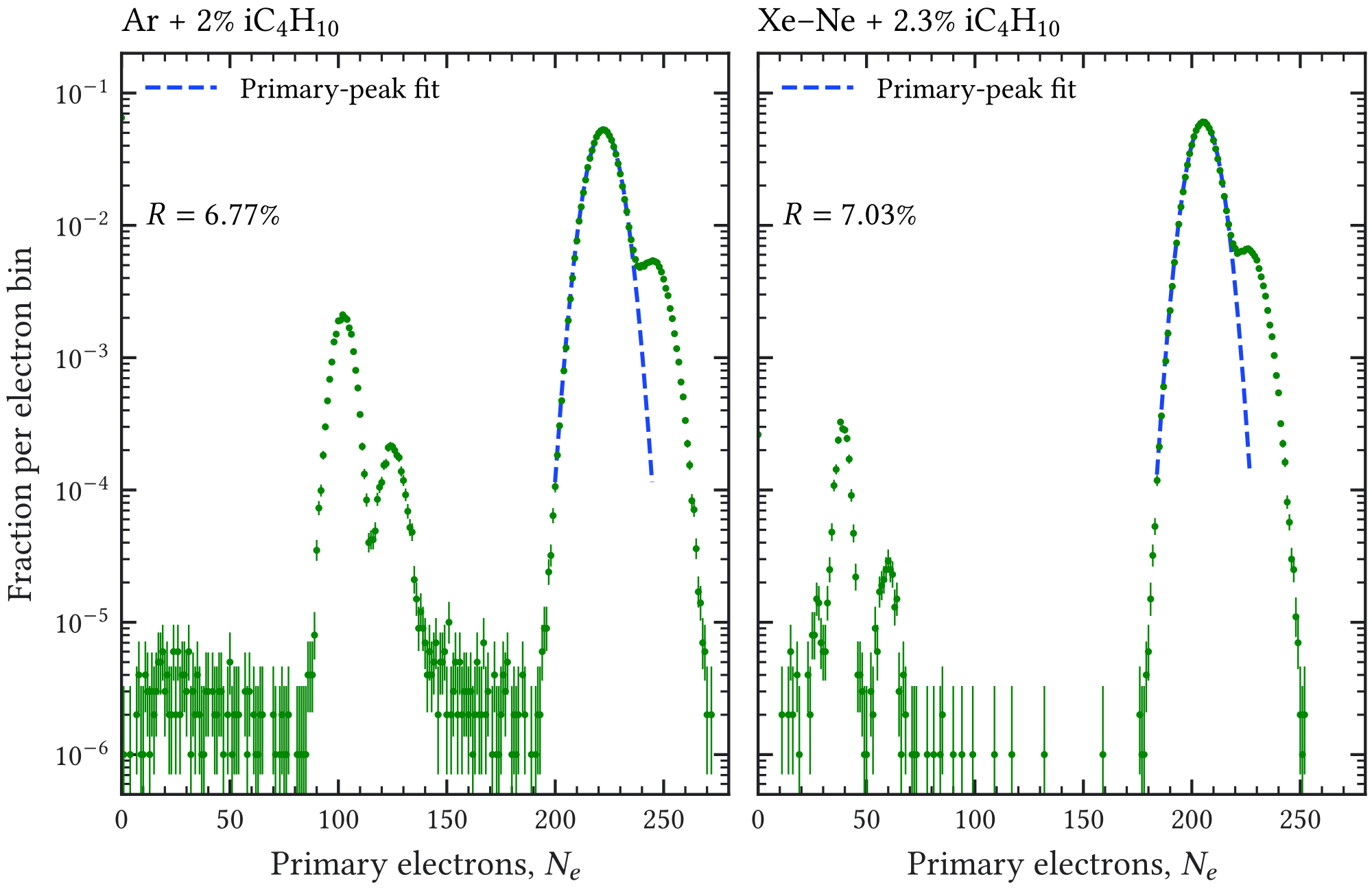
Equation (3.10) separates the primary-ionization and avalanche contributions from electronic noise, which becomes increasingly important near threshold. The approximately $7 %$ primary-only FWHM in Figure 3.4 is an intrinsic reference for these gas mixtures and this X-ray energy. It excludes amplification, charge loss and readout fluctuations and therefore is not the predicted resolution of the complete detector. Measured microbulk resolutions also depend on gain and collection conditions [72].

Avalanche ultraviolet photons can initiate secondary avalanches by photoionizing gas species or releasing electrons from surfaces. Adding isobutane suppresses this feedback through absorption and non-radiative molecular relaxation. The quencher also changes charge transport, as illustrated in Figure 3.5.

Figure 3.5: Effect of the isobutane quencher fraction on Micromegas gas-transport properties, computed with Garfield++ / Magboltz gas tables at 20 ∘ C [ 70 ]. The upper row shows argon–isobutane mixtures and the lower row shows equal-partial-pressure xenon–neon mixtures with isobutane. The curves are plotted as a function of the reduced drift field in bar units, 𝐸 𝑑 / 𝑝 . The vertical dotted line in each row marks the representative operating point used to read the transport properties in the detector-response studies: the center of the 𝐸 𝑑 ≃ 133 – 153 V / cm range at 𝑝 = 1.4 bar for the argon mixtures, and 𝐸 𝑑 ≃ 111 V / cm at 𝑝 = 1.05 bar for the xenon–neon mixture. The 2 % argon–isobutane curve is a representative detector-response scan rather than the frozen background-model gas: the conservative IAXO-D1 reference in Section 6 uses argon–isobutane at 1 % , while the 2.3 % xenon–neon–isobutane mixture belongs to the separate BabyIAXO response studies. — Figure 3.5: Effect of the isobutane quencher fraction on Micromegas gas-transport properties, computed with `Garfield++`/`Magboltz` gas tables at $20^{\circ} C$ [70]. The upper row shows argon–isobutane mixtures and the lower row shows equal-partial-pressure xenon–neon mixtures with isobutane. The curves are plotted as a function of the reduced drift field in bar units, $𝐸_{𝑑} / 𝑝$ . The vertical dotted line in each row marks the representative operating point used to read the transport properties in the detector-response studies: the center of the $𝐸_{𝑑} ≃ 133$ – $153 V / cm$ range at $𝑝 = 1.4 bar$ for the argon mixtures, and $𝐸_{𝑑} ≃ 111 V / cm$ at $𝑝 = 1.05 bar$ for the xenon–neon mixture. The $2 %$ argon–isobutane curve is a representative detector-response scan rather than the frozen background-model gas: the conservative IAXO-D1 reference in Section 6 uses argon–isobutane at $1 %$ , while the $2.3 %$ xenon–neon–isobutane mixture belongs to the separate BabyIAXO response studies.

Increasing the isobutane fraction generally reduces transverse diffusion in these scans, producing a narrower cloud after the same drift distance. Changes in drift velocity and longitudinal diffusion also affect the relation between waveform timing, drift position, and the extent of a localized ionization cluster. The dotted lines mark reference operating fields, rather than gas-optimization boundaries. Gas choice must therefore balance charge transport, attachment, amplification stability, and operational requirements. The calculation workflow is described in Section 4.6.6.

3.1.3 Micropattern Gaseous Detectors: Micromegas

Micromegas (MICRO-MEsh GAseous Structure) detectors are micropattern gaseous detectors in which a thin metallic mesh separates the drift region from a narrow amplification gap [73]. Ionization electrons produced in the drift volume pass through the mesh when the field ratio between amplification and drift regions is favorable, and then avalanche in the high-field gap before being collected by the anode strips. This separation between a relatively low-field drift volume and a very high-field amplification region gives Micromegas detectors fast signals, good spatial granularity, and stable operation at gains suitable for soft X-ray detection.

For axion helioscopes and other rare-event searches, the relevant implementation is the microbulk Micromegas. In this technology the mesh, insulating pillars, and readout pattern are manufactured from copper-clad kapton using photolithographic processes, producing a thin and mechanically uniform amplification structure [74]. The small material budget, the use of radiopure copper and kapton, and the possibility of producing fine two-dimensional strip readouts are central advantages for low-background X-ray detectors. They also make the detector naturally compatible with a TPC analysis strategy: X-ray events produce compact clusters, while tracks from cosmic rays or radioactive backgrounds tend to be more extended in at least one strip projection.

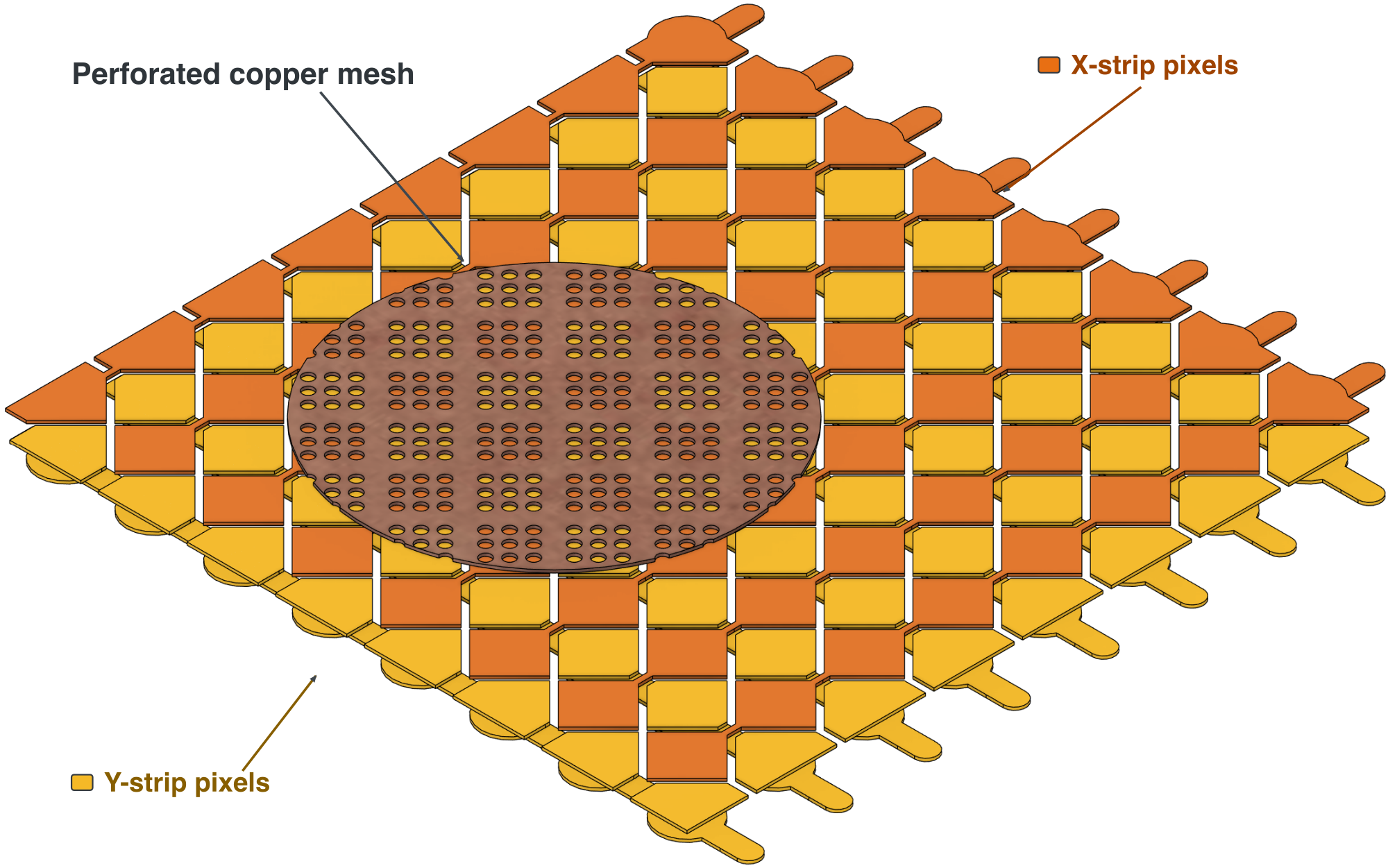
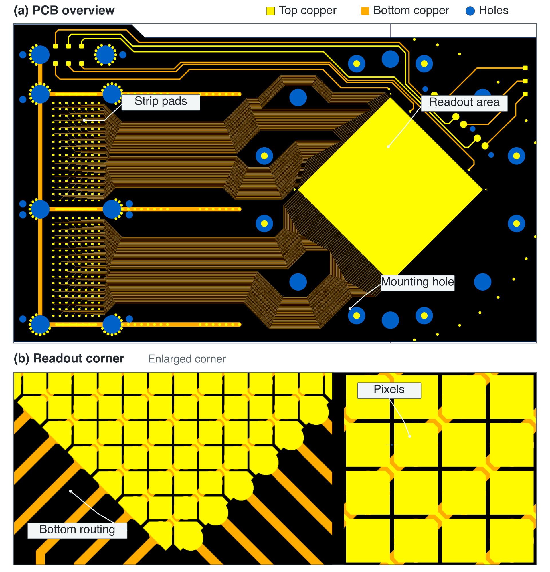
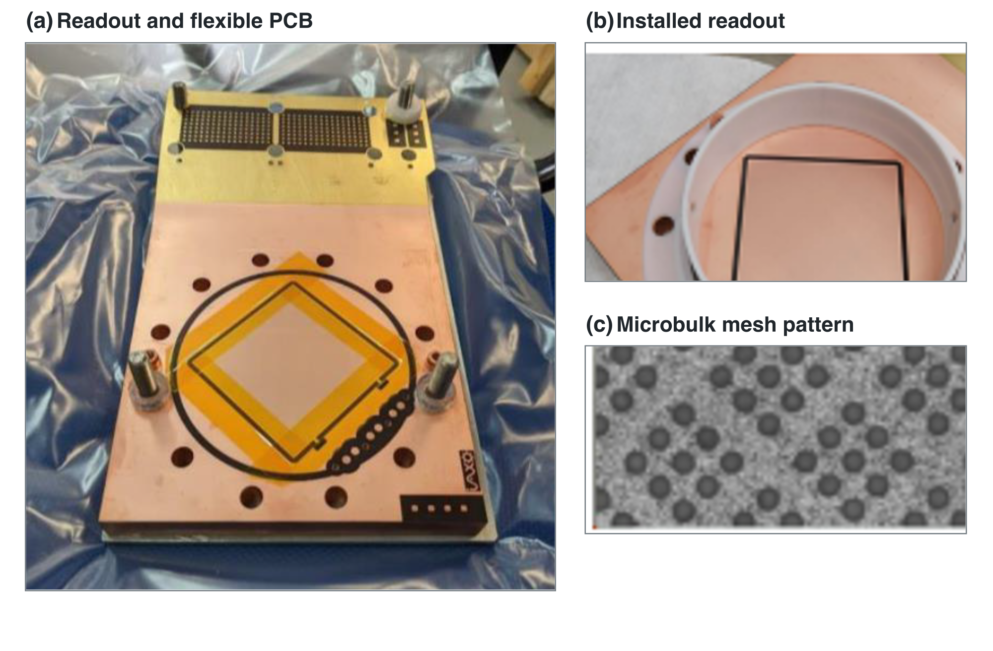
Three distinct length scales should not be conflated. The $6 cm$ -wide IAXO readout contains 120 strips per coordinate, giving a strip pitch of $500 mum$ . At each X–Y strip crossing, the IAXO-D1 mesh photograph shows a $3 \times 3$ group of microscopic openings. Microbulk structures of this detector family use holes of order $40 mum$ in diameter on an approximately $100 mum$ triangular pitch, while the etched polyimide defines an amplification gap of approximately $50 mum$ [56, 72]. The strip pitch sets the two-dimensional readout granularity; the much smaller hole pitch and gap determine electron transmission and avalanche formation.

The operating point of a Micromegas detector is defined by the drift field, mesh voltage, gas mixture, pressure, and readout threshold. The mesh transparency must be high enough that primary electrons enter the amplification gap efficiently, while the gain must be large enough to resolve keV deposits without approaching unstable discharge conditions. These two requirements are coupled: the field ratio controls electron focusing through the mesh, while the amplification field controls both signal size and discharge probability. Consequently, stable operation is not only a matter of setting a high voltage, but of choosing a consistent gas, voltage, and electronics configuration and monitoring it through calibration data.

The combination of radiopurity, segmentation, low threshold, and successful operation in CAST makes microbulk Micromegas the baseline detector technology for the IAXO Micromegas line [12, 16, 40].

Figure 3.6: Simplified design of a microbulk Micromegas readout, showing the orthogonal X and Y strip pixels and a cut-out of the perforated copper mesh above them. The design is based on the BabyIAXO readout in Figure 3.10 , but it contains 8 + 8 strips instead of 120 + 120 . The X-strip pixels are connected in the same PCB layer, while the Y-strip pixels are connected through the bottom layer. In the real detector, the mesh is separated from the readout by an approximately 50 mum amplification gap; the full TPC drift region lies above the mesh and is not shown. — Figure 3.6: Simplified design of a microbulk Micromegas readout, showing the orthogonal X and Y strip pixels and a cut-out of the perforated copper mesh above them. The design is based on the BabyIAXO readout in Figure 3.10, but it contains $8 + 8$ strips instead of $120 + 120$ . The X-strip pixels are connected in the same PCB layer, while the Y-strip pixels are connected through the bottom layer. In the real detector, the mesh is separated from the readout by an approximately $50 mum$ amplification gap; the full TPC drift region lies above the mesh and is not shown.

3.2 The BabyIAXO Micromegas Detector Prototypes

The baseline detector technology for IAXO and BabyIAXO is the microbulk Micromegas. Its successful operation in CAST, where it provided low-background X-ray detection for the solar-axion search, makes it the established baseline choice for the IAXO program.

The TPC design of the BabyIAXO Micromegas detector remains similar to the CAST Micromegas detectors, since both experiments are designed with the same goal of detecting solar axions. The gas volume is a cylinder with a diameter of $10 cm$ and a height of $3 cm$ , with a total volume of $235.62 {cm}^{3}$ . The microbulk micromegas readout has a square shape with a side of $6 cm$ . The readout has 120 strips for each direction, for a total of 240 channels.

The full $6 \times 6 {cm}^{2}$ readout is not the signal-normalization area targeted by the frozen conservative background analysis. Earlier reconstruction studies integrated readout energy or required a hit centroid inside a $15 mm$ -radius central circle, representing a broad entrance/optics footprint. The background-analysis-v2-conservative-reference contract instead selects the calibrated maximum reconstructed track and requires its paired X–Y center to satisfy $𝑟 < 10 mm$ . This gives the explicit signal area $𝐴_{fid} = 𝜋 {cm}^{2}$ . An energy integrated inside a readout region and a containment decision on the reconstructed track are physically different observables; the background-model chapter keeps the older $15 mm$ results as auxiliary studies rather than treating the two fiducial definitions as equivalent.

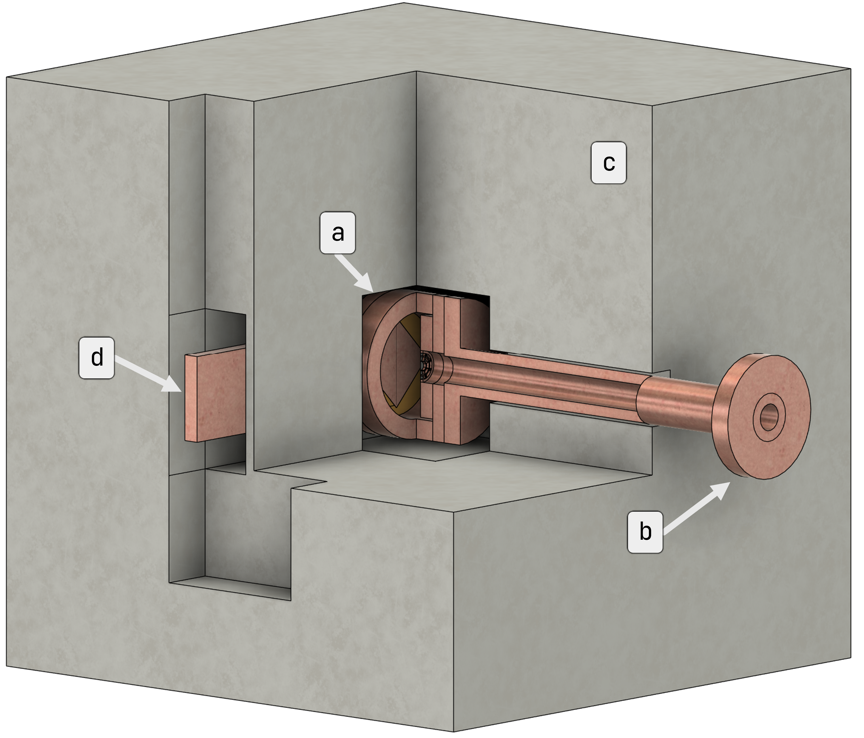
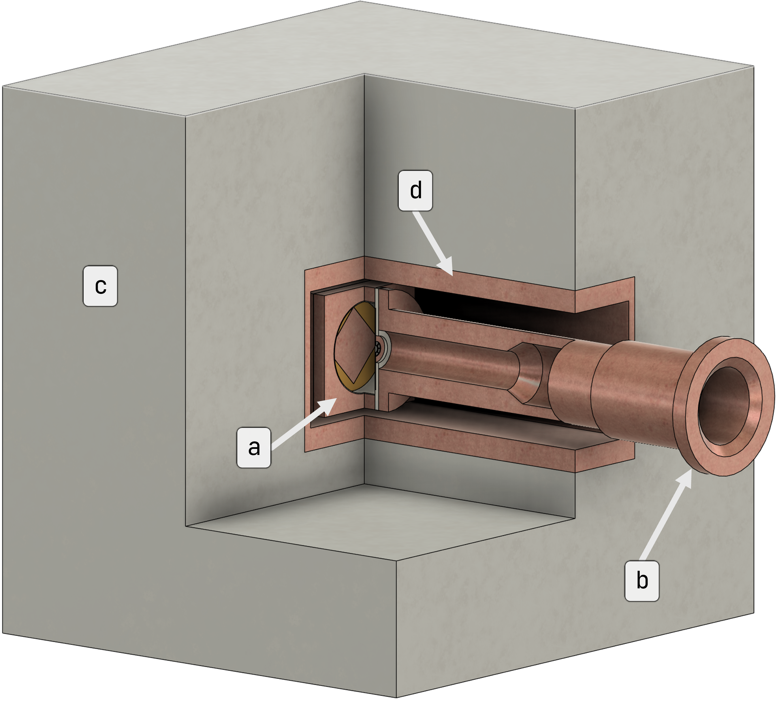
There are two distinct generations of detector prototypes: IAXO-D0 and IAXO-D1. Both prototypes share the same core design scale, including TPC dimensions, readout size, number of strips, and nominal lead-shielding thickness. The main differences are in the chamber and pipe design, shielding serviceability, Micromegas PCB implementation, and electronics.

Feature	IAXO-D0	IAXO-D1
Role	Late CAST-derived detector used for Zaragoza prototype campaigns, veto tests, and simulation validation.	BabyIAXO-oriented prototype focused on integration, serviceability, and updated electronics.
Chamber and shielding	Cylindrical chamber, brick-based lead shielding, and protruding copper backplate.	Square-footprint chamber, thicker pipe, movable lead shielding, and inner copper liner.
Readout integration	Rigid readout connection through flat cables to a combined FEC–Feminos unit.	Flexible Micromegas PCB and front-end placement closer to the readout to reduce cable length.
Electronics emphasis	AGET front-end chips with Feminos back-end electronics.	STAGE front-end chips with ARC-compatible back-end electronics.
Thesis use	Experimental benchmark for waveform, calibration, and veto-coincidence studies.	Quantitative argon reference geometry in this thesis and precursor to the separate BabyIAXO projection.

Table 3.1: Operational comparison of the IAXO-D0 and IAXO-D1 Micromegas prototypes discussed in this chapter.

(a) IAXO-D0: cylindrical chamber, brick shielding, and laterally protruding copper backplate.

(b) IAXO-D1: square chamber, movable monolithic shielding, thicker pipe, and inner copper liner. — (a) IAXO-D0: cylindrical chamber, brick shielding, and laterally protruding copper backplate.

3.2.1 IAXO-D0

The IAXO-D0 prototype is, in essence, the latest CAST-derived design. The chamber is cylindrical, with a large copper backplate that protrudes laterally from the shielding. The copper pipe is thinner in the middle and the shielding is made of lead bricks. In order to access or move the detector, the lead shielding must be partially removed brick by brick. The front-end electronic chips are four AGET chips and the back-end electronics is a Feminos card [75]. The front-end and back-end electronics are physically connected into a single FEC–Feminos unit, which is connected to the readout through flat cables.

A significant data-taking campaign was performed with the IAXO-D0 prototype in Zaragoza using the same Micromegas detector that had operated in CAST, shortly after it was decommissioned. This campaign validated the detector and tested the prototype veto system, with emphasis on the reduction of cosmic-ray-induced background. Earlier measurement campaigns with the same prototype family were also performed using other Micromegas detectors from the same generation [60]. Together, these measurements provided the experimental anchor for the simulation and background-rejection studies developed later in the thesis.

3.2.2 IAXO-D1

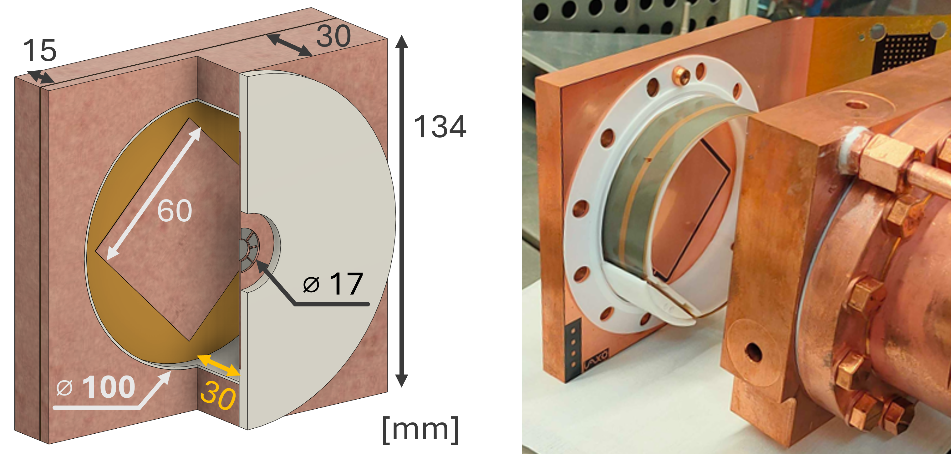
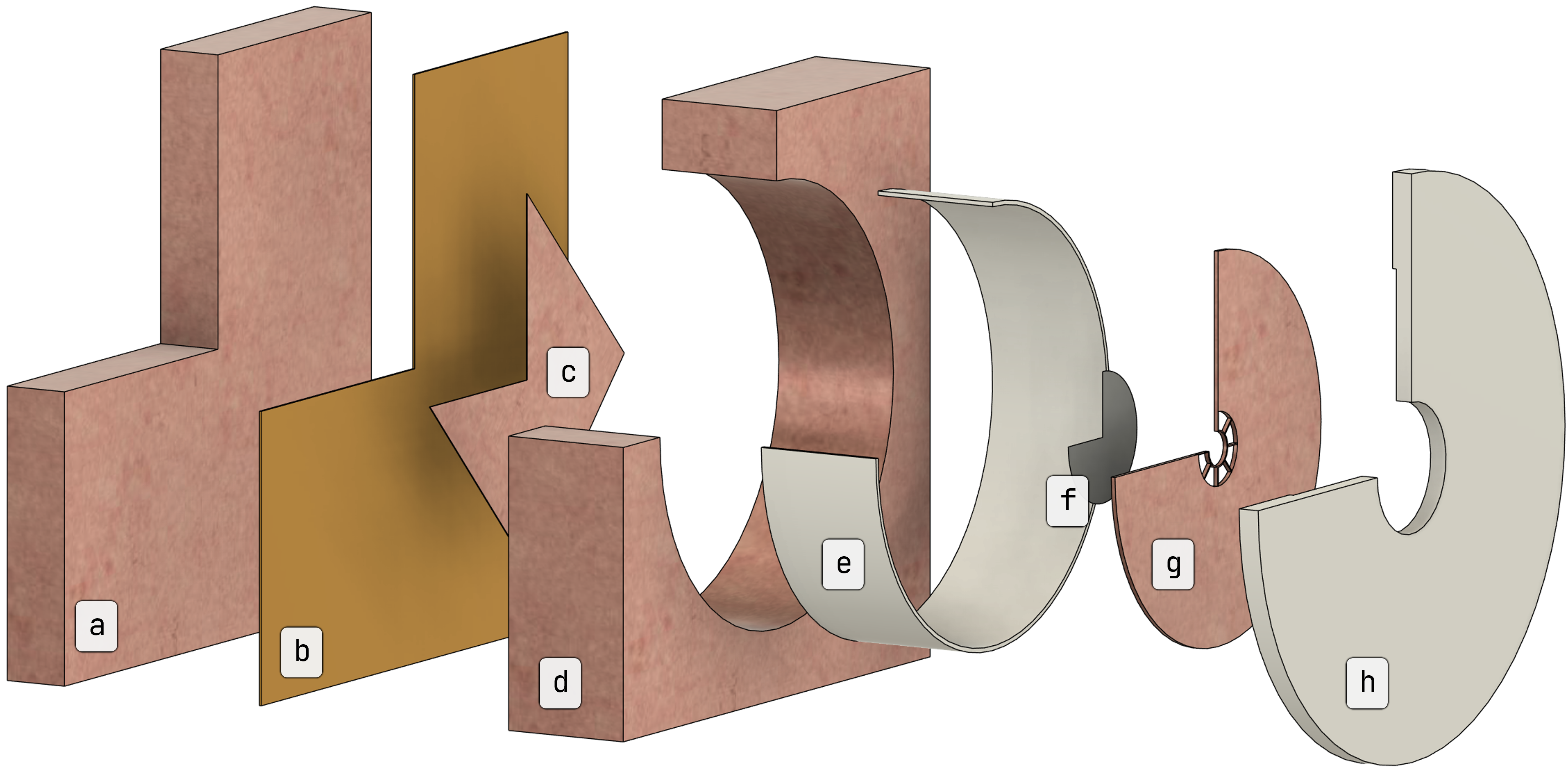
The IAXO-D1 prototype introduces significant improvements with respect to IAXO-D0. The shielding is a lead box with a square shaft in the middle. It is designed to sit on linear rails so that it can be moved laterally to access the detector, substantially reducing the time required for service operations. The chamber has a square footprint and the copper pipe is significantly thicker. The Micromegas PCB can be bent to fit the shielding aperture, and the readout strips exit the shielding hole in parallel to the pipe.

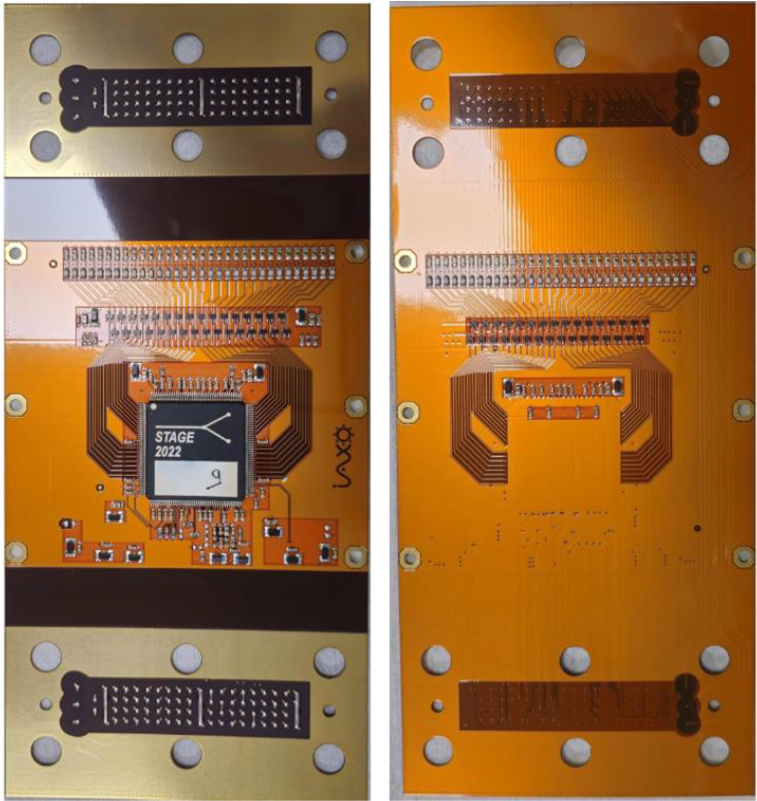
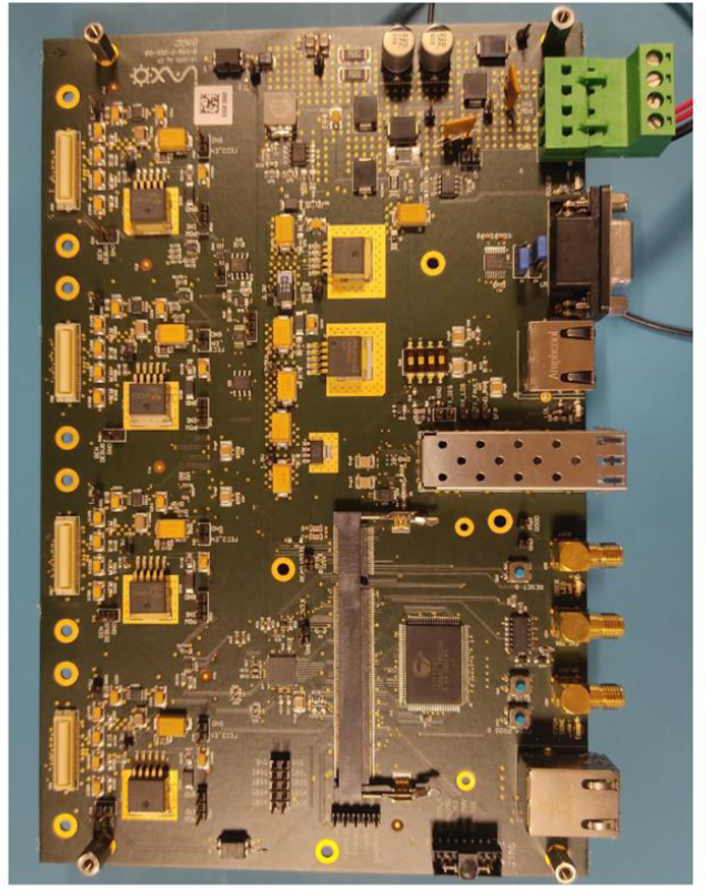
The front-end electronics are based on four STAGE chips, while the back-end electronics follow an ARC-compatible design. The STAGE front-end cards (Figure 3.12(a)) are placed inside the shielding next to the readout. This minimizes the capacitance and noise pickup of the low-level analog connection. Radiopurity requirements distinguish the flexible PCB substrate from its mounted components: the March 2025 electronics report lists radiopure FEC substrates but does not classify the populated cards as fully radiopure [76]. The component inventory and assay status therefore remain relevant to the material-background model. The ARC-compatible back-end (Figure 3.12(b)) contains substantially more conventional, non-radiopure components and is therefore kept outside the passive shield, where it is also accessible for power, control, data transfer, and maintenance [76]. Flexible interconnects carry the digitized and control signals through the shielding penetration.

Figure 3.8: IAXO-D1 detector chamber. The left image shows the simplified geometry as used in the simulations and the right image shows a picture of the actual chamber. The electric field shaper ring can be seen in the outside of the PTFE liner. The gas lines (two, one not shown) can be seen running in parallel to the pipe. The chamber backplate and body are fastened to the pipe with 12 copper bolts.

Figure 3.9: Exploded view of the IAXO-D1 detector chamber created using the simplified simulation geometry from Figure 3.8 . The copper backplate (a), readout PCB (b), readout/mesh (c), chamber copper walls (d), chamber inner PTFE lining (e), ultra-thin aluminized mylar window (f), conductive copper cathode support (g), and PTFE cathode support (h) are shown. In practice, the cathode parts (f, g, h) are glued together into a single piece. The whole PCB (b) is coated in copper, as seen in Figure 3.8 , in order to provide a uniform electric field in the TPC; only the area inside the TPC is connected to high voltage. — Figure 3.9: Exploded view of the IAXO-D1 detector chamber created using the simplified simulation geometry from Figure 3.8. The copper backplate (a), readout PCB (b), readout/mesh (c), chamber copper walls (d), chamber inner PTFE lining (e), ultra-thin aluminized mylar window (f), conductive copper cathode support (g), and PTFE cathode support (h) are shown. In practice, the cathode parts (f, g, h) are glued together into a single piece. The whole PCB (b) is coated in copper, as seen in Figure 3.8, in order to provide a uniform electric field in the TPC; only the area inside the TPC is connected to high voltage.

Figure 3.10: IAXO-D1 Micromegas PCB reconstructed by combining its Gerber layers. Panel (a) shows the complete PCB: top-copper features are yellow, bottom-copper routing is orange, and mounting holes are blue. The connector pads for the 240 strips are grouped on the left, while the square active readout occupies the center-right. Panel (b) shows an enlarged and rotated readout corner. The yellow pixels are arranged in orthogonal strips, with one strip direction connected through the bottom copper layer. The simplified model in Figure 3.6 is based on this design.

Figure 3.11: IAXO-D1 microbulk Micromegas readout. Panel (a) shows the readout and its flexible PCB extension before installation, panel (b) shows the square active area installed in the chamber, and panel (c) is an optical-microscope close-up of the perforated copper mesh. The close-up resolves the 3 × 3 hole group associated with each 500 mum -pitch strip crossing. — Figure 3.11: IAXO-D1 microbulk Micromegas readout. Panel (a) shows the readout and its flexible PCB extension before installation, panel (b) shows the square active area installed in the chamber, and panel (c) is an optical-microscope close-up of the perforated copper mesh. The close-up resolves the $3 \times 3$ hole group associated with each $500 mum$ -pitch strip crossing.

(b) Back-end electronics. — (a) Front-end card (FEC).

The IAXO-D1 spatial response was measured independently with the SOLEIL synchrotron X-ray beam [77]. For a $90 mum \times 90 mum$ beam at $6 keV$ and a drift field of $100 V {cm}^{- 1}$ , Gaussian fits to the reconstructed event-centroid distributions gave standard deviations slightly below $100 mum$ in both views. This is a centroid-resolution measurement, including finite beam size and the stated event selection; it is not the strip pitch or the width of an individual ionization cloud. Charge sharing permits centroid reconstruction finer than the $500 mum$ strip pitch. The measured energy and field dependence provides an existing constraint on diffusion and reconstruction modeling, while the different beamline and laboratory noise conditions must be retained in comparisons.

3.3 Detector Ancillary Systems

3.3.1 Gas system

The IAXO Micromegas prototypes can operate with argon–isobutane or xenon–neon–isobutane mixtures. Argon with $2 %$ isobutane at $1.4 bar$ was used for most CAST operation [12], while equal-partial-pressure xenon and neon with $2.3 %$ isobutane was used during its final years [40]. The xenon–neon mixture avoids the argon escape structure near the signal region and the intrinsic $^{39} Ar$ contribution, but its cost favors closed-loop purification and recirculation.

Recirculation reduces noble-gas consumption, but it also turns the chamber, pipework, pump, buffer volume, valves, and filters into a coupled contamination system. Leaks, outgassing, and radon emanation can then accumulate activity that an open flow would continuously remove. This is not only a gas-quality issue: IAXO-D1 measurements have shown that the low-gain alpha rate changes markedly between open-loop and recirculating configurations, motivating dedicated radon-source checks and purification studies [78]. Closed-loop operation therefore requires both chemical purification and radiological control of the complete circulation path.

For detector response, the important quantities are mixture composition, pressure, temperature, drift field, flow stability, and gas purity. These parameters determine the charge-transport properties summarized earlier and must match the gas tables used in simulation. The Garfield++/Magboltz workflow is described in Section 4.6.6; the prototype piping, open- and closed-loop implementation, and safety provisions are documented in Appendix Section A.2, including the full-page diagram in Figure A.2.

3.3.2 High voltage and slow control

Separate cathode and mesh channels establish the drift and amplification fields. Their stability affects electron transport, mesh transparency, gain, and reconstructed topology, while the independently biased veto photomultiplier tubes determine the veto threshold and timing response. Controlled ramping, current monitoring, filtering, and trip handling are therefore part of the detector-response contract.

The slow-control layer records these settings together with gas and environmental conditions and supports remote intervention during long runs. The reusable hvps control library developed in this thesis is described in Section 4.7.3. The prototype power-distribution and Node-RED implementation details [79] are retained in Appendix Section A.2.

3.4 Shielding and Veto Systems

The Micromegas detector is only one part of the complete low-background detection line. For BabyIAXO, the detector must operate inside a passive shield and in coincidence with an active veto system, so the mechanical envelope, signal feedthroughs, calibration access, gas services, high-voltage routing, and data-acquisition interfaces all have to remain compatible with the surrounding shielding. The detailed passive-shielding studies, cosmic-ray-induced background simulations, and scintillator–cadmium veto design are therefore treated in the dedicated shielding and veto chapter, Section 5. In the present chapter, the relevant point is the interface: Micromegas operation defines the X-ray-like event selection, timing reference, calibration strategy, and veto-coincidence information that the background model uses later.

3.5 Data Acquisition System

This section describes the detector-facing DAQ hardware: how the Micromegas strips and veto channels are connected to front-end electronics, back-end timing, and the DAQ computer. The acquisition software itself, including the feminos-daq refactor and online viewer, is treated in the software chapter.

The Data Acquisition (DAQ) system is responsible for the readout and storage of the detector signals. It is composed of three main components: the Front-End Card (FEC), the Front-End Module (FEM), and the Data Acquisition Computer (DAQ PC).

The overall architecture follows the same detector-readout philosophy adopted for the IAXO pathfinder line at CAST, where the 240 Micromegas strips were read through four AGET chips connected to a Feminos back-end board, with the external muon-veto signal routed to an otherwise unused AGET channel so that veto and TPC information could be recorded together on an event-by-event basis [80]. In this sense, the pathfinder operation serves as a practical bridge between the late CAST Micromegas generation and the more scalable BabyIAXO-oriented readout concepts.

Figure 3.13: Acquisition-chain schematic for the Micromegas TPC and active veto system, adapted from the CAST pathfinder readout concept described in Cristina Margalejo Blasco’s thesis [ 80 ]. The diagram represents the commissioned IAXO-D0 prototype layout, in which the TPC and veto signals are handled by separate AGET/Feminos branches that share a timing reference before event building. The IAXO-D1 and final BabyIAXO implementations use distinct STAGE/ARC-oriented electronics and should not be inferred from this hardware diagram. This synchronized two-branch structure is what allows Micromegas waveform observables and veto-coincidence information to be compared later within the same event-by-event analysis chain. — Figure 3.13: Acquisition-chain schematic for the Micromegas TPC and active veto system, adapted from the CAST pathfinder readout concept described in Cristina Margalejo Blasco’s thesis [80]. The diagram represents the commissioned IAXO-D0 prototype layout, in which the TPC and veto signals are handled by separate AGET/Feminos branches that share a timing reference before event building. The IAXO-D1 and final BabyIAXO implementations use distinct STAGE/ARC-oriented electronics and should not be inferred from this hardware diagram. This synchronized two-branch structure is what allows Micromegas waveform observables and veto-coincidence information to be compared later within the same event-by-event analysis chain.

Figure 3.13 is intentionally placed before the detailed hardware subsections because it summarizes the logic that connects the detector electronics to the later data analysis. At acquisition level, the important point is not only that the Micromegas strips are digitized, but that their waveforms are recorded in a timing-aware event structure that can also accommodate veto information. This common event record is what later allows one to compare Micromegas pulse-shape observables, reconstructed X-ray candidates, and veto coincidences within the same analysis chain. In other words, the DAQ architecture already encodes part of the future discrimination strategy.

The commissioned IAXO-D0 chain uses four AGET front-end chips for the 240 Micromegas strips and a Feminos module for configuration, timing, readout control, and Ethernet transfer [75, 81]. Multiple boards can be synchronized through a common Trigger Clock Module, allowing the TPC and veto branches to be assembled into a timing-aware event record. The board architecture, register-level configuration, and UDP data path are documented in Appendix Section A.2. The feminos-daq refactor, ROOT output, compression, online monitoring, and event viewer are described in Section 4.7.2.

3.5.1 Run configuration and waveform observables

At the detector-operation level, the relevant point is how a run is configured and how the digitized waveform encodes the quantities used later in reconstruction and monitoring. A typical acquisition with the FEC–Feminos chain proceeds as follows:

An instance of the acquisition software is started on the DAQ PC. The software is configured with the IP addresses of the Feminos boards and the desired acquisition settings.

The start sequence is initiated by the operator. The software sends the configuration commands to the Feminos boards to set the AGET chips to the desired settings, including the power-up sequence of the AGET chips.

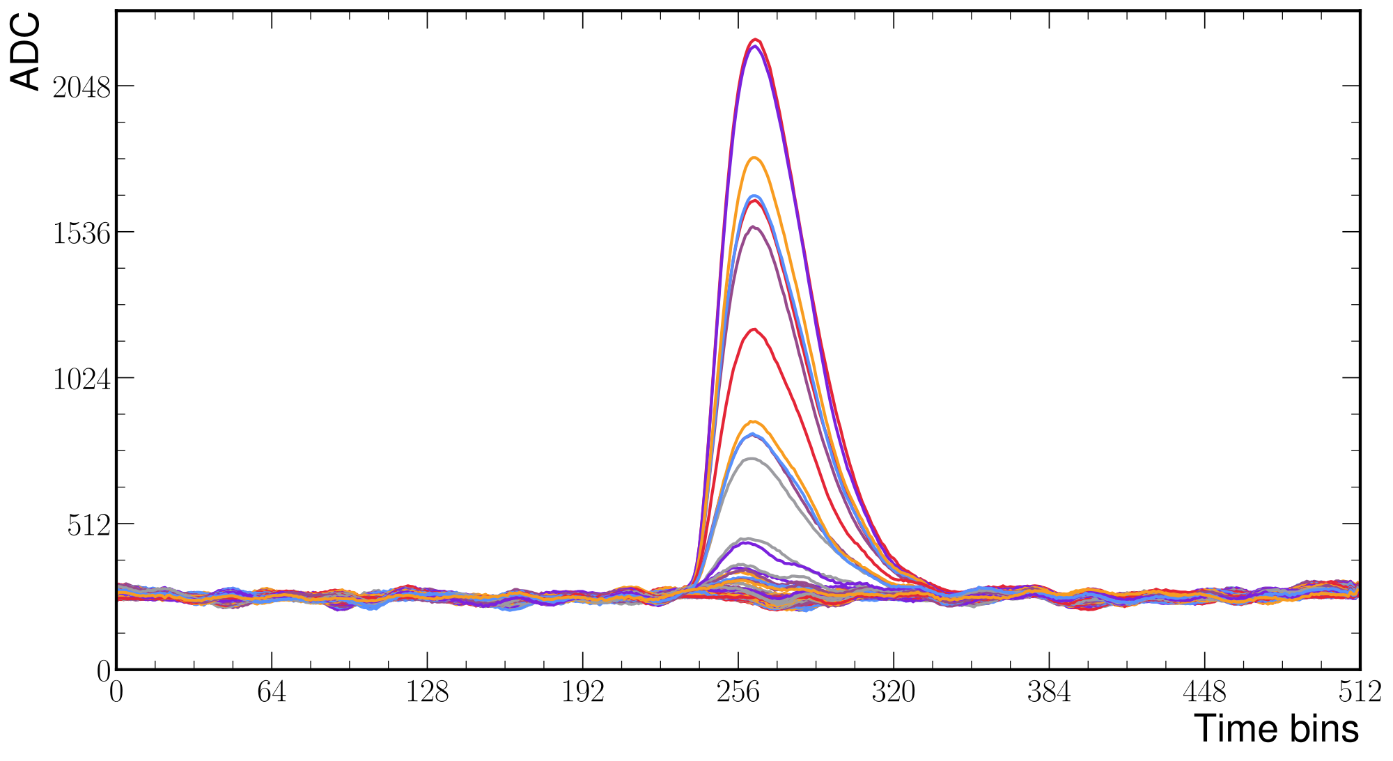
Figure 3.14: IAXO-D0 55 Fe calibration event sample. Showing all 240 channels with the same base level due to the pedestal subtraction. — Figure 3.14: IAXO-D0 $^{55} Fe$ calibration event sample. Showing all 240 channels with the same base level due to the pedestal subtraction.

A pedestal run is performed to measure the mean $𝑚_{𝑖}$ and standard deviation $𝜎_{𝑖}$ of the channels when they are not triggered. The pedestal values are stored internally in the Feminos boards and are subtracted from the signal values during data acquisition, so that all signals have the same base level. This base level, corresponding to zero signal, can be set in the configuration and is usually set to 250 ADC counts, as recommended by the Feminos authors. Figure 3.14 shows a sample event with all channels at the same base level due to the pedestal subtraction.

Each channel can serve as a trigger. The trigger level, the value above which a signal is considered a trigger, can be configured and is set to three times the standard deviation of the pedestal values. The acquisition can be configured to return all signals or only the triggered signals.

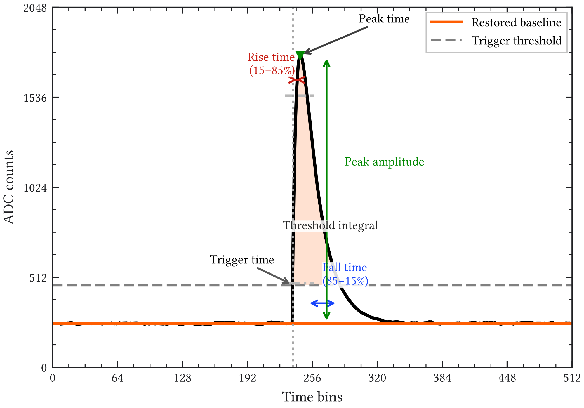
Figure 3.15: Representative single-channel Micromegas waveform after pedestal subtraction. The channel is characterized by the restored baseline, trigger threshold, peak amplitude and peak time, rise and fall times, and the threshold integral. These waveform-level quantities are the building blocks from which the later event-level observables used in the signal analysis are derived.

Figure 3.15 summarizes the morphology of a typical single-channel waveform after pedestal subtraction. The relevant information is the pulse height, the collected charge, the time at which the pulse develops, and the width and symmetry of the shaped response. These quantities are not only electronics diagnostics: they are the first experimental handles used to separate compact X-ray-like events from extended tracks, pile-up, or pathological waveforms.

The most important run settings are therefore those that modify this pulse morphology. The gain sets the overall amplitude scale, the shaping time determines the width and asymmetry of the pulse, the sampling period fixes the time granularity of the waveform, and the trigger delay determines how much pre-trigger baseline and post-trigger tail are recorded. The trigger threshold also matters because it decides which channels enter the event and can therefore affect both the reconstructed charge and the timing pattern. Although some settings can in principle be adjusted channel by channel, they are normally chosen coherently for the full readout so that the event can be interpreted with a single response model.

After digitization, the reconstruction combines the channel-level pulse information into a smaller set of event-level quantities. For calibration, these are mainly energy estimators, such as the pulse height, the integrated charge around the maximum, the charge above threshold, or the reconstructed readout energy. For event selection, they are complemented by timing and topology descriptors that measure whether the active strips are compact and mutually synchronous. This is the level at which the raw waveform description becomes part of the later signal analysis: X-ray-like events should produce narrow, well-aligned strip responses, whereas background-like or poorly reconstructed events tend to be broader, more asymmetric, or less synchronous.

3.6 Detector Calibration

The operation of a Micromegas detector involves a set of coupled parameters that must remain under control in order to guarantee stable gain, reproducible energy calibration, and a well-defined trigger threshold. In the gas system, the most relevant settings are the gas flow, chamber pressure, and gas mixture. In the detector itself, the drift and amplification voltages determine the transparency of the mesh and the gas gain. At the readout level, shaping time, trigger delay, sampling configuration, and threshold settings define how the pulse is digitized and which events are retained. In addition to these explicitly configured quantities, environmental variables such as temperature, as well as slow drifts in gas quality, can also modify the detector response. For that reason, the relevant detector and DAQ settings are stored together with the run metadata and are monitored through regular calibration runs.

From the point of view of data taking, the acquisition is organized in runs, each one corresponding to a period with fixed detector and DAQ settings. The run duration may range from a few minutes to several hours depending on the purpose of the measurement. In practice, the most important distinction is between calibration runs and background or tracking runs. The former provide a controlled X-ray-like reference with which the detector gain, energy scale, resolution, and threshold can be monitored. The latter provide the physics data used for background characterization and, when relevant, for axion-sensitive exposure. In the CAST pathfinder campaign, the daily operating sequence was explicitly structured around this logic, with regular $^{55} Fe$ calibrations used to track the detector response and to associate each background or tracking period with the most representative nearby calibration [80].

3.6.1 Standard X-ray calibration

The standard calibration procedure uses a source of soft X rays placed in front of the detector window, typically through a dedicated calibration port. The most common choice is $^{55} Fe$ , whose dominant manganese K-shell line at $5.9 keV$ lies inside the energy region most relevant for the axion search and generates compact, X-ray-like events in the gas. Additional sources such as $^{109} Cd$ may be used for complementary checks at higher energy, but $^{55} Fe$ remains the reference source for routine operation. Since photons in this energy range interact predominantly through the photoelectric effect, the resulting signal is a localized ionization cluster that closely resembles the topology of a low-energy X-ray conversion in the Micromegas gas.

In routine operation, the calibration data are first used for a fast data-quality check. A reconstructed hit map verifies that the source illuminates the expected region of the detector and that no large-scale asymmetry or dead area has appeared. The corresponding energy spectrum is then inspected to verify the position and width of the main photopeak, which provides an immediate monitor of gain stability, energy resolution, and effective threshold. This daily quick-look procedure was an important part of the CAST pathfinder operation and is especially relevant for surface-running detectors, where small changes in gas quality, voltage settings, or noise conditions can translate into visible shifts of the calibration peak from run to run [80]. Figure 3.16 compares a representative IAXO-D0 $^{55} Fe$ spectrum with a simulated spectrum after fitting their energy scales separately and broadening the reconstructed simulated energy to the measured main-peak width. The dominant structure is the manganese $𝐾_{𝛼}$ line at $5.9 keV$ , while the weaker $𝐾_{𝛽}$ contribution appears at higher energy. The fit includes both manganese lines, and the quoted FWHM refers to the fitted $𝐾_{𝛼}$ component. The fixed $𝐾_{𝛽} / 𝐾_{𝛼}$ intensity ratio is applied to the integrated Gaussian areas, with the widths scaled as the square root of energy.

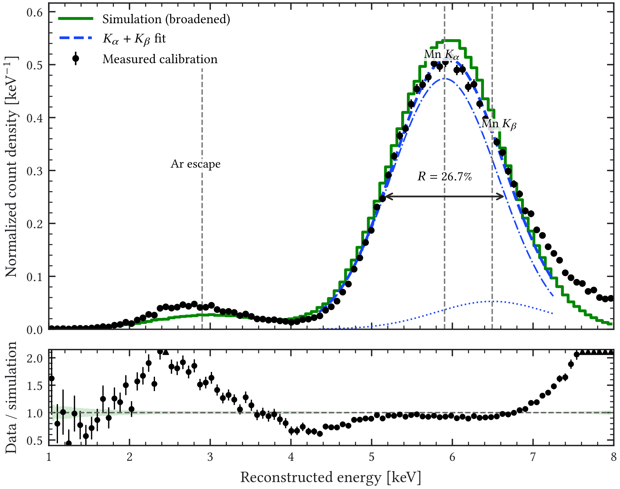
Figure 3.16: Measured and simulated 55 Fe calibration spectra for an IAXO-D0 run, shown after anchoring the dominant line to 5.9 keV . The unit-area densities use 0.071 keV -wide bins and contain 80,669 measured and 900,000 simulated entries. Black error bars and the green band show the respective per-bin statistical uncertainties at 68.27% coverage; normalization-induced bin correlations are not shown. The lower panel gives the data-to-simulation ratio, with the simulation uncertainty shown around unity; triangles mark values outside the displayed ratio range. The simulation receives an additional Gaussian broadening of the scalar reconstructed energy, fitted to the measured main-peak width; the resulting agreement in that width is imposed rather than predicted by the detector-response chain. The blue fit contains the manganese 𝐾 𝛼 and 𝐾 𝛽 contributions; the annotation gives for the 𝐾 𝛼 component. — Figure 3.16: Measured and simulated $^{55} Fe$ calibration spectra for an IAXO-D0 run, shown after anchoring the dominant line to $5.9 keV$ . The unit-area densities use $0.071 keV$ -wide bins and contain 80,669 measured and 900,000 simulated entries. Black error bars and the green band show the respective per-bin statistical uncertainties at 68.27% coverage; normalization-induced bin correlations are not shown. The lower panel gives the data-to-simulation ratio, with the simulation uncertainty shown around unity; triangles mark values outside the displayed ratio range. The simulation receives an additional Gaussian broadening of the scalar reconstructed energy, fitted to the measured main-peak width; the resulting agreement in that width is imposed rather than predicted by the detector-response chain. The blue fit contains the manganese $𝐾_{𝛼}$ and $𝐾_{𝛽}$ contributions; the annotation gives
for the $𝐾_{𝛼}$ component.

The energy calibration itself is obtained from fits to the reconstructed calibration spectrum. For argon-based mixtures, the main $5.9 keV$ photopeak and the argon escape structure around $2.9 keV$ provide two anchors for calibrating ADC units to deposited energy [80]. For xenon-based operation, the $5.9 keV$ line supplies only a one-point scale if a zero intercept is assumed; additional lines or calibrated charge injection are required to test linearity and determine an offset. Repeating the applicable procedure run by run makes it possible to quantify gain evolution and to propagate the calibration constants to associated physics runs and selection studies.

The reconstructed calibration energy can be estimated in several ways, each one emphasizing a different aspect of the waveform or of the reconstructed hit. Table 3.2 compares a representative set of these energy estimators using the same calibration run. Integrated charge-like quantities give comparable resolutions, while a single-channel maximum-amplitude estimator performs significantly worse because it is more sensitive to charge sharing and local fluctuations. The comparison uses measured data alone so that differences between estimators are not obscured by separately fitted simulation broadening.

Energy estimator	Measured FWHM / centroid
Reconstructed readout energy	$26.6 %$
Peak-neighborhood charge	$26.7 %$
Sum of channel pulse heights	$26.6 %$
Charge above threshold	$28.1 %$
Full-window charge	$29.4 %$
Largest channel pulse height	$50.1 %$

Table 3.2: Energy resolution obtained from selected energy estimators in the same measured

^{55} Fe

calibration run. The resolution is defined as the fitted

𝐾_{𝛼}

FWHM divided by the

𝐾_{𝛼}

centroid. Each estimator is scaled by its main-peak centroid, and the final two-line fit uses

4.75 – 6.75 keV

, as in the displayed spectrum. These fitted widths characterize this run and fit convention.

The display broadening in Figure 3.16 is separate from the detector-hit smearing applied before reconstruction in the production response. Neither a fitted centroid nor a fitted scalar width establishes waveform-level closure or the energy dependence of the selection efficiency. Measured traces contain correlated residual structure that can alter threshold crossings and peak multiplicity. The data-driven raw-signal emulation developed to address this limitation, including its implementation and validation status, is presented as a computational contribution in Section 4.5.

3.6.2 UV-light calibration R&D

A complementary calibration concept was explored during a three-month internship at CEA Saclay. This work is not part of the baseline BabyIAXO calibration strategy, which remains based on X-ray source runs, but it is worth retaining as detector R&D because it addresses a closely related problem: how to generate controlled, localized, and time-stamped primary electrons in a Micromegas gas volume. The idea is inspired by Micromegas-based photocathode detectors such as PICOSEC [82], where ultraviolet photons release photoelectrons that are subsequently drifted and amplified.

In the CEA setup, a pulsed ultraviolet source illuminated an aluminized cathode through a UV-transparent window. The lamp trigger provided a timing reference, while the anode pulse arrival time was measured after electron drift and amplification. By repeating the measurement with spacers of different thicknesses, the drift distance was changed in a controlled way and the drift velocity could be estimated from the variation of pulse arrival time with distance. The presentation study used argon–isobutane mixtures, several quencher fractions, and comparisons with Garfield++/Magboltz drift-velocity calculations. The measured velocities had the expected order of magnitude and qualitative field dependence, although offsets with respect to the simulation remained and were attributed to possible gas-settling, field, photocathode, or space-charge effects.

For the present thesis, the importance of this work is methodological rather than as a mature calibration proposal. A pulsed UV system could, in principle, provide single-electron or few-electron calibration, localized topological checks, timing studies, and gas-transport measurements without relying only on radioactive X-ray sources. However, the tested gas-discharge lamp had limited pulse stability, and a quantitative implementation for BabyIAXO would require a better-controlled UV source, calibrated photocathode response, stable gas conditions, and a dedicated comparison with the final detector geometry and readout. Supplementary figures from this R&D study are collected in Appendix Section A.3.