Experimental Typst web edition · Veto chapter pilot
A Veto-System Validation and Supplementary Performance
A.1 Supplementary interaction plots for detector and veto design
The evaluated-data comparisons below supplement the design discussion in the veto-system chapter. They test constituent cross-section inputs for BC408 scintillator and cadmium; they do not by themselves validate moderation times or detector response.
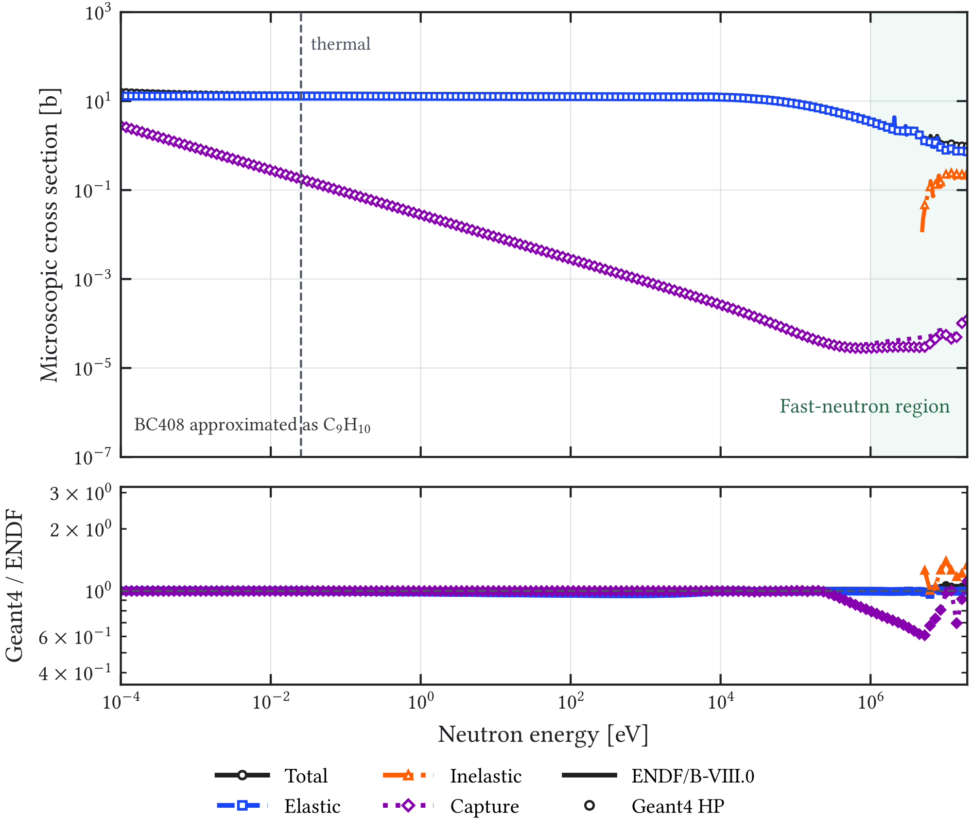
Geant4 high-precision neutron cross sections for BC408, approximated as . The comparison tests consistency of the constituent-weighted elastic, capture, and inelastic input data. It does not test bound-hydrogen thermal scattering, secondary energy–angle distributions, or the full moderation-time response.The reference curves use ENDF/B-VIII.0 MF=3 pointwise cross sections. BC408 is approximated as polyvinyltoluene, , with atom-fraction-weighted carbon and hydrogen contributions; cadmium uses natural isotope abundances. The Geant4 points use G4NDL4.6 for version 11.0.3 and the same channel grouping as the natural-lead comparison in Section A.2.
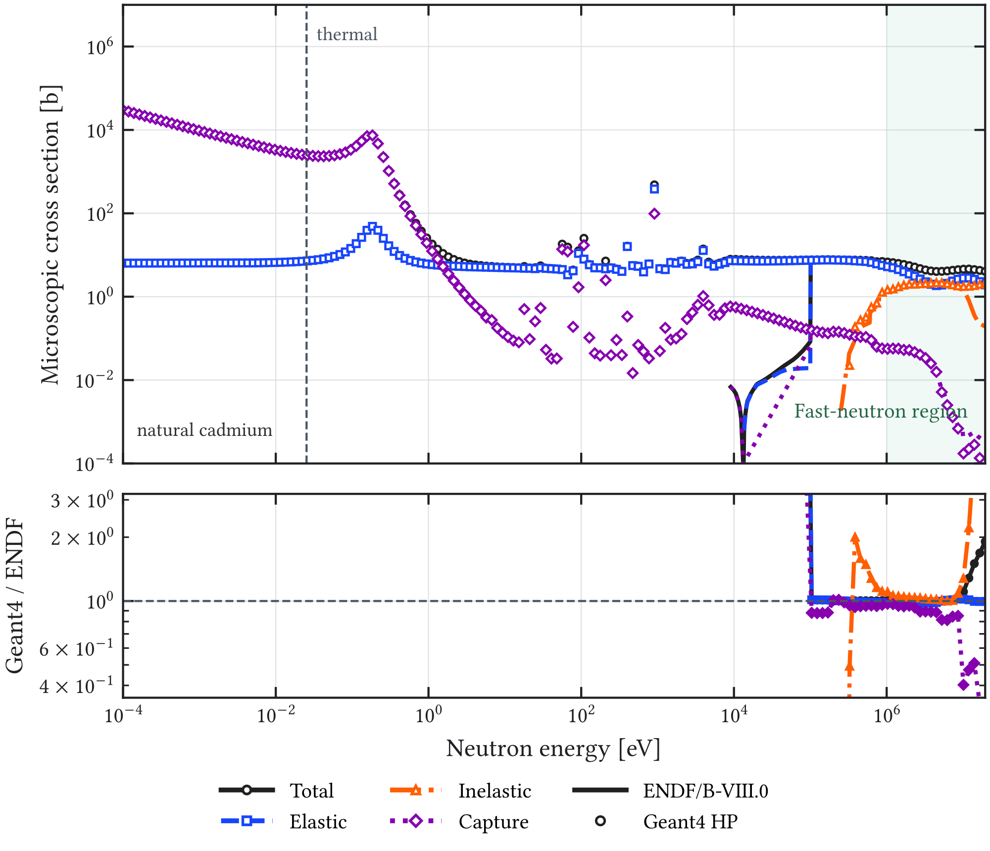
Geant4 high-precision neutron cross sections for natural cadmium. The large thermal and epithermal capture cross section motivates cadmium layers next to scintillator. The emitted gamma cascade is prompt relative to capture; moderation and transport can delay the capture relative to the initiating event.A.2 Detailed veto-physics validation
The main veto chapter retains only the conclusions of the nuclear-data and detector-response validation. This section records the evaluated-data comparisons, physics-model choices, and operating-point diagnostics needed to reproduce those conclusions. They test selected transport inputs and quantify the response variation among the configurations examined. Their scope is narrower than a complete detector-response validation or a measurement of the BabyIAXO background level.
A.2.1 High-precision neutron data
Natural-lead reference curves were constructed from ENDF/B-VIII.0 evaluations by weighting , , , and by their natural abundances [128]. The corresponding Geant4 points were extracted from the G4NDL4.6 high-precision tables used by Geant4 11.0.3 [129, 130]. Elastic, inelastic, capture, and channels were compared with the same isotope weights.
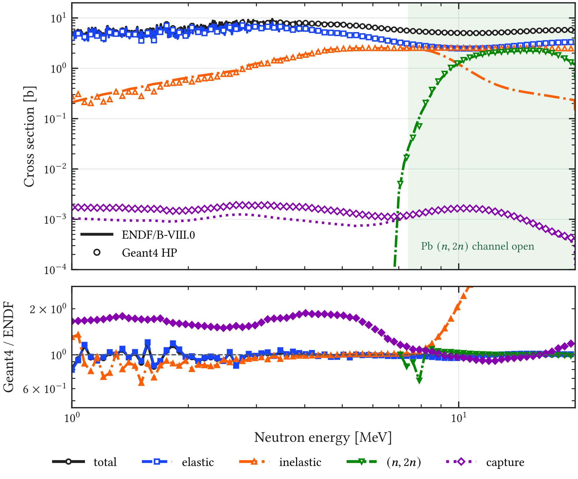
Geant4 11.0.3. The comparison isolates the transport input from detector-geometry effects.The same construction for PVT-like BC408 and natural cadmium is shown in Figure A.1 and Figure A.2. Those comparisons check the evaluated elastic and capture inputs relevant to moderation in scintillator and capture in the cadmium sheets. Constituent-weighted cross sections do not test the thermal-scattering law , which describes energy and momentum transfer to bound atoms. The installed thermal-scattering process, material mapping, temperature, and data must therefore be recorded separately before assigning a moderation-time uncertainty. A useful comparison holds the geometry and source fixed and compares the available bound-hydrogen treatment with the free-gas approximation, examining the capture-time distribution and the fraction reconstructed inside the veto window.
A.2.2 Secondary-neutron production in lead
Interaction probabilities do not determine the energy and angle of the emitted secondary neutrons. A thin-target benchmark was therefore performed against the EXFOR natural-lead double-differential data of Takahashi et al. at [131, 132]. The reported integral uses and ; the experimental spectra are tabulated at – angle centers within those bin edges. Each model used incident neutrons on a natural-lead target.
| Model | Integrated production cross section [b] | Model/EXFOR |
|---|---|---|
| EXFOR Takahashi et al. | 5.875 | 1.000 |
QGSP_BIC_HP | 5.358 | 0.912 |
QGSP_BERT_HP | 5.404 | 0.920 |
FTFP_BERT_HP | 5.392 | 0.918 |
Shielding | 5.381 | 0.916 |
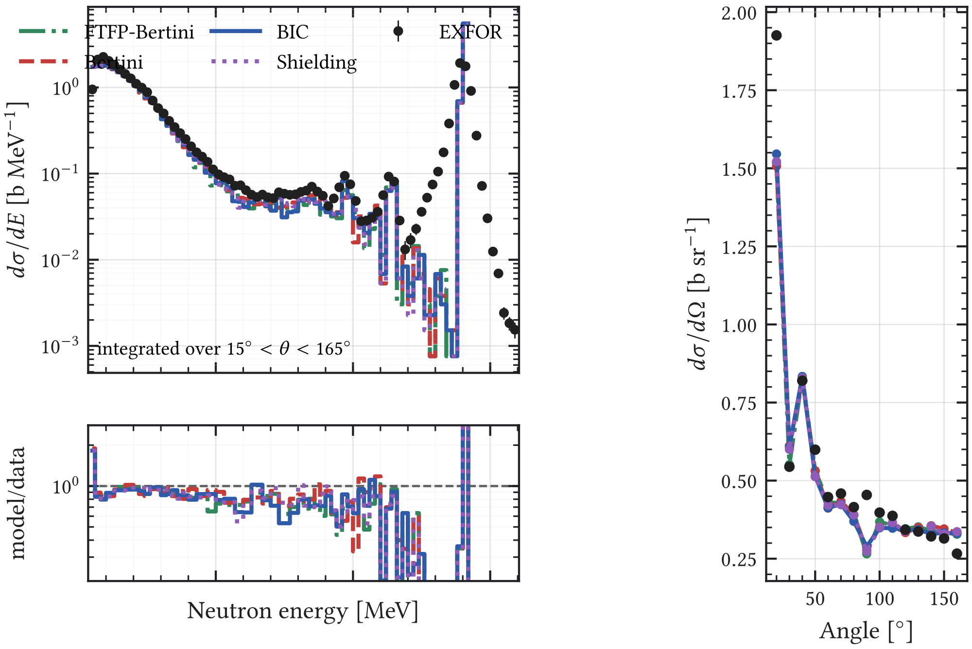
The comparison supports the low-energy shower interpretation but does not validate the full GeV-scale HENSA response. At higher energy, cascade-model differences must be assessed in the detector geometry and treated as a model envelope.
A.2.3 Cadmium capture-gamma response
A natural-cadmium sheet is effectively opaque to thermal neutrons but is not a fast-neutron shield. Its role is to capture neutrons after moderation and emit a gamma cascade close to active scintillator.
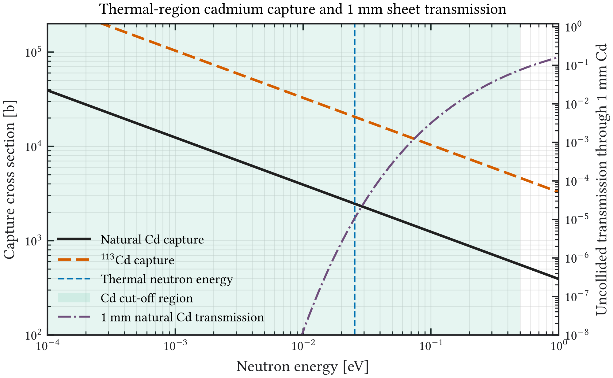
The REST interface forwards strict-isotope and PhotonEvaporation options to G4ParticleHPManager before the neutron processes are constructed. The default and strict-ParticleHP variants give and photons per cadmium capture and and of emitted gamma energy per capture. The PhotonEvaporation variant gives photons and per capture, while suppressing the overproduced line.
![Figure A.6: Evaluated 113 Cd prompt-gamma lines compared with the PhotonEvaporation cascade in the HENSA three-layer geometry [ 133 ]. The histogram is normalized per simulated cadmium capture.](assets/ca0bfbe072a77d74c8cfd118.png)
PhotonEvaporation cascade in the HENSA three-layer geometry [133]. The histogram is normalized per simulated cadmium capture.| Line window | IAEA yield | Simulated yield | Simulation/IAEA |
|---|---|---|---|
| 0.7375 | 0.9019 | 1.22 | |
| 0.1420 | 0.0394 | 0.28 | |
| 0.0531 | 0.0156 | 0.29 | |
| 0.00472 | 0.00101 | 0.21 | |
| 0.00305 | 0.00058 | 0.19 |
PhotonEvaporation. Individual line yields differ from the evaluated values by factors ranging from to , including discrepancies of about a factor five. The model is therefore used only to test aggregate cascade-response sensitivity, not for line-spectroscopy predictions.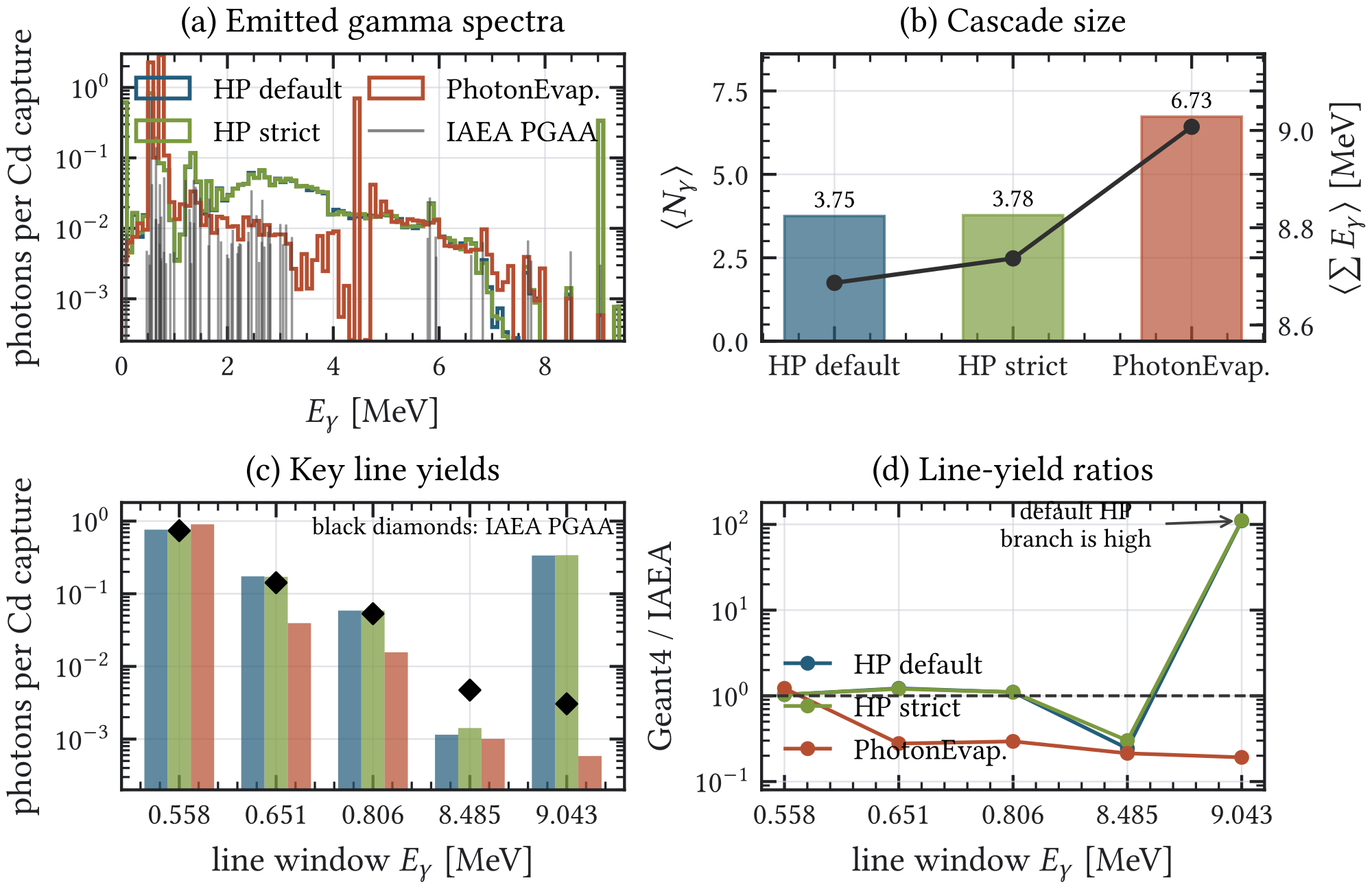
PhotonEvaporation preserves the total emitted-energy scale while shifting the cascade toward more numerous, lower-energy photons.The corresponding detector-response replay separates the approximately stable probability of reconstructing any veto peak from the more model-dependent fixed-energy thresholds.
| Peak-level criterion | defaultParticleHP | strictParticleHP | PhotonEvaporation |
|---|---|---|---|
| Any reconstructed veto peak | |||
| equiv. | |||
| equiv. |
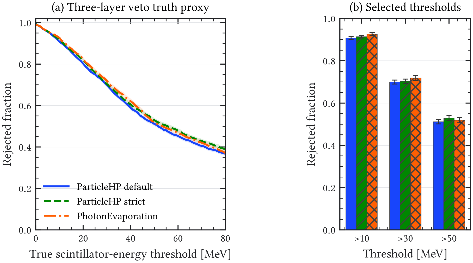
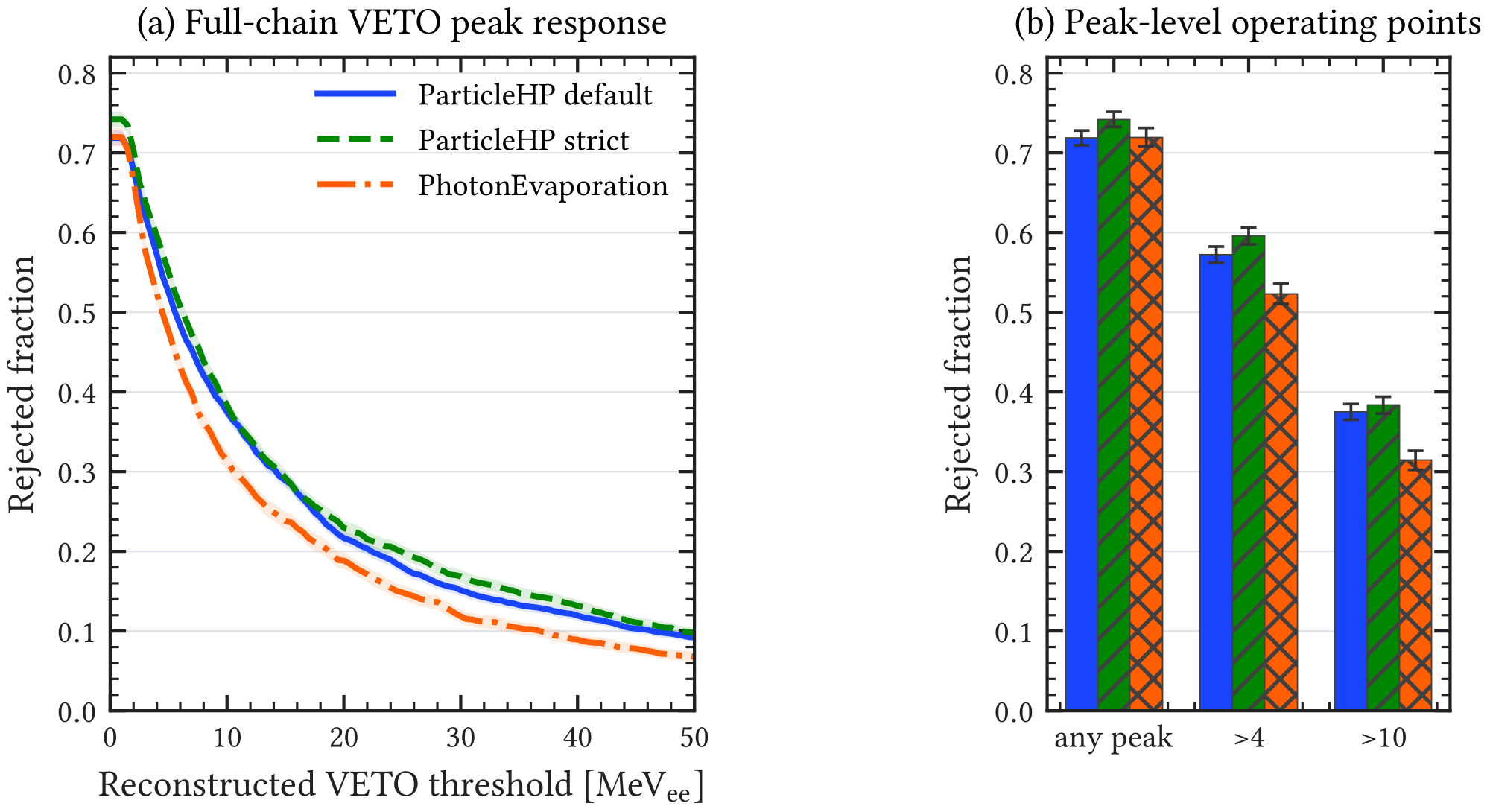
PhotonEvaporation cascade reduces fixed reconstructed-energy rejection.The observed spread is an envelope of the tested cascade models, not a confidence interval on the true response. For a design decision, each variant must be propagated through the same frozen selector and the same layer geometries; stability of the any-peak probability alone does not establish stability of a classifier dominated by reconstructed energy. The evaluated-cascade approach implemented in G4CASCADE provides a further benchmark candidate [134]. Its published validation used a different Geant4 version, so compatibility with the present Geant4 11.0.3 stack and the required capture isotopes must be checked before using it as a replacement model.
A.3 Tracking-orientation systematic
BabyIAXO changes inclination during solar tracking. To test the resulting source-direction acceptance, the three-layer detector geometry was held fixed while the incident source direction was rotated over to . The scan used the same source and reconstruction settings at every point.
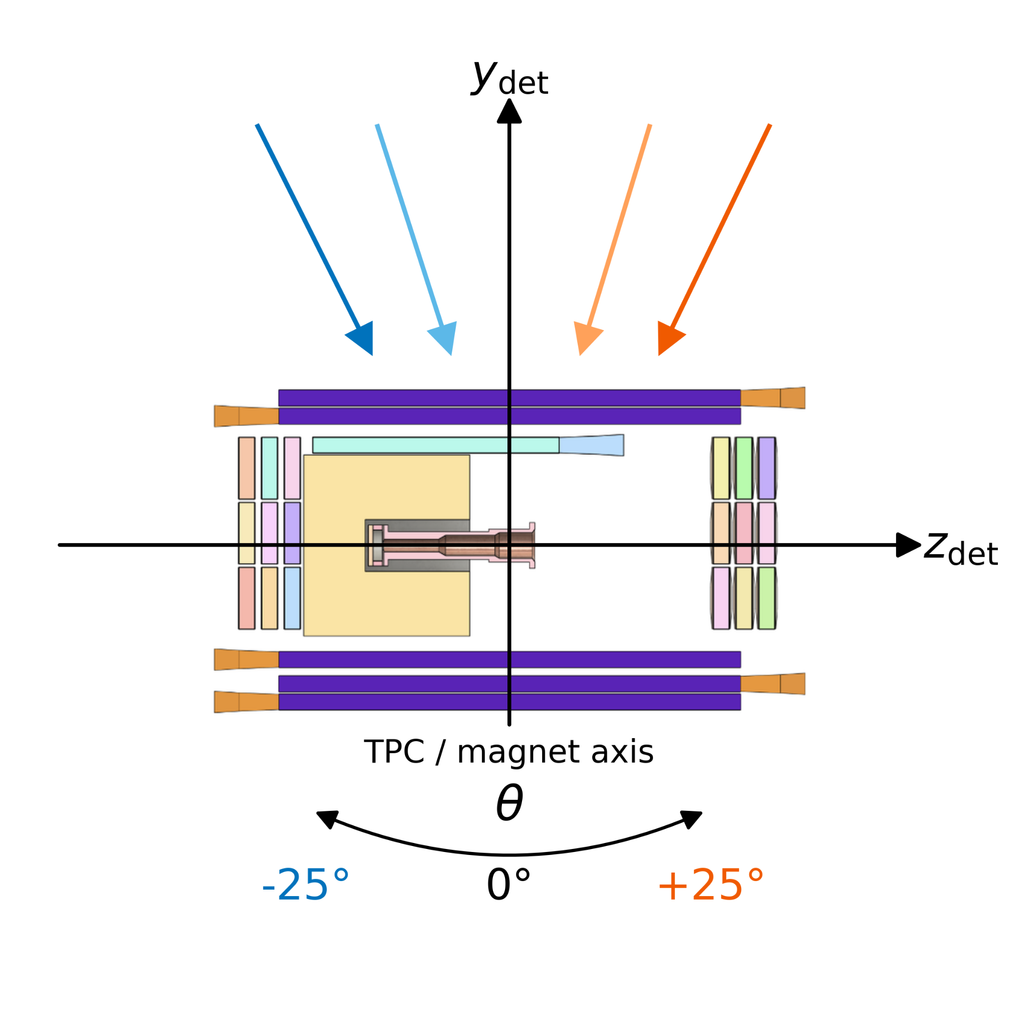
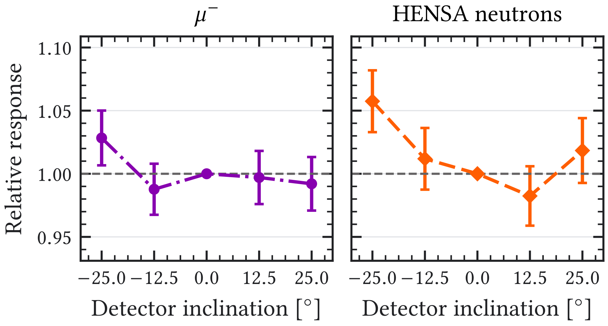
The neutron response ranges from to , and the muon response from to , relative to the horizontal configuration. No monotonic dependence is resolved within this scan. The horizontal geometry is therefore an adequate reference for the tested source prescription, although the corrected source-angle convention must be propagated before transferring this conclusion to the final tracking response.
A.4 Supplementary waveform and selection diagnostics
The main chapter retains the simulation-derived capture-retention plot and the aggregate selector result. This section records the complementary timing and accidental-selection diagnostics.
The capture-history input contains 57,799 records in cadmium-sheet regions. The retention curve is conditional on the 55,581 records with ; this requirement excludes 2217 pre-trigger records and one record at or beyond . Here is measured relative to the first simulated gas deposit and is therefore a trigger proxy rather than a reconstructed acquisition time. The cumulative , , and values at 50, 70, and use those 55,581 records as their denominator. They integrate from zero delay to the stated upper boundary and must not be interpreted as the acceptance of the reconstructed – delayed interval. Specifically, of the physical records occur at , whereas fall in . The truncated-exponential maximum-likelihood fit uses 39,532 records in and gives . An independent bootstrap that resamples the 2659 capture-bearing analysis entries, keeping captures from each entry together, gives a central 68% statistical interval of –, consistent with the profile-likelihood result. This check accounts for correlations within an analysis entry; it does not include transport-model uncertainties or establish independence of entries sharing an unavailable primary-history identifier.
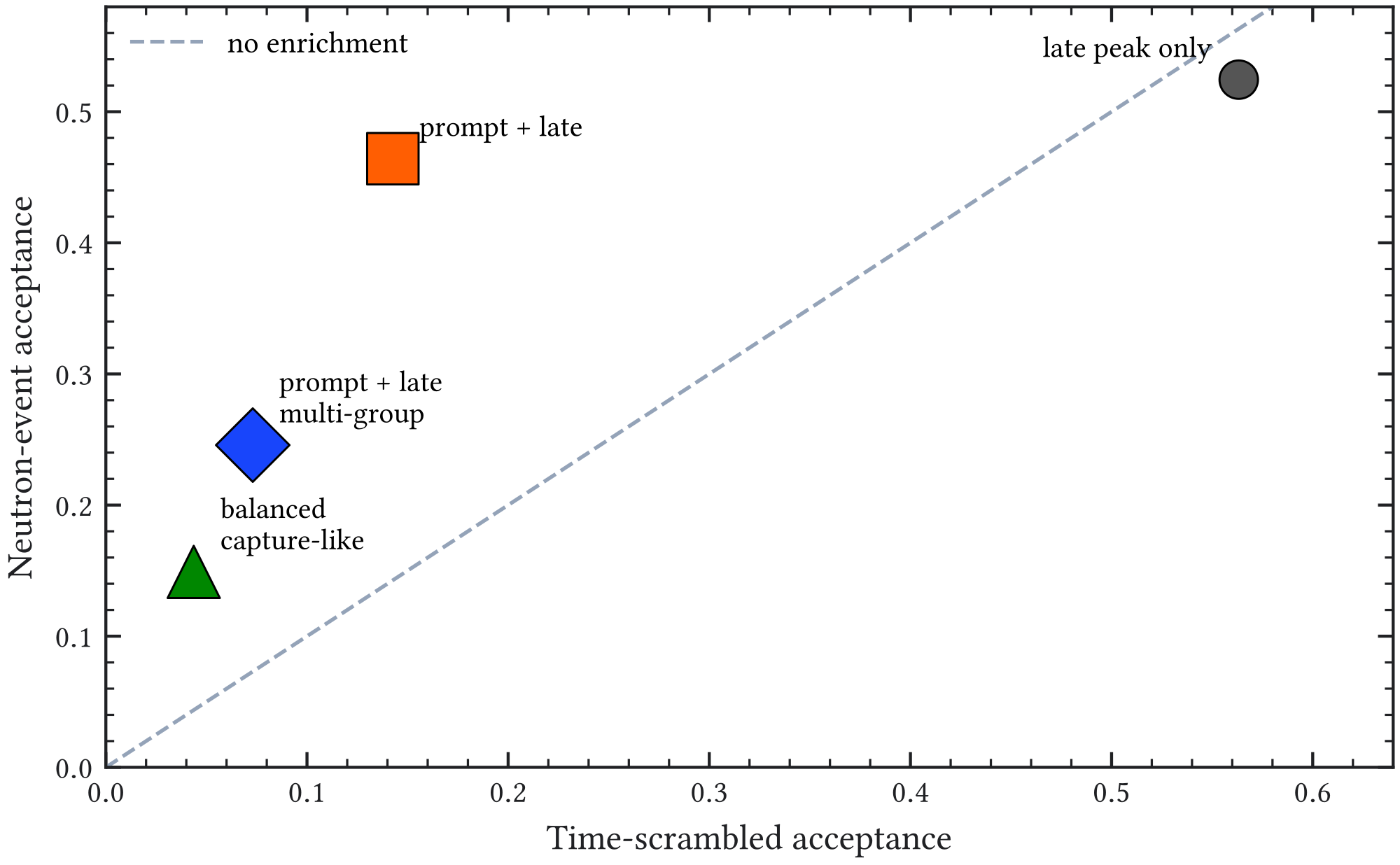
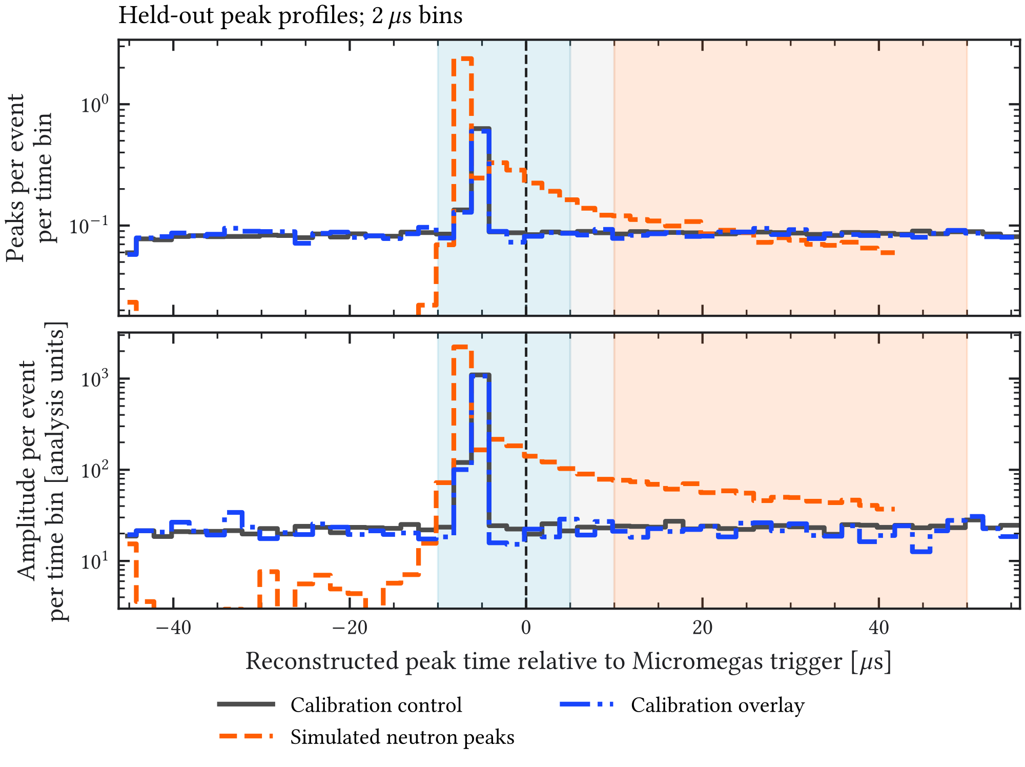
An event-mixing study time-scrambles simulated neutron veto trains relative to the Micromegas trigger. The quantitative comparison is summarized in Section 5; the figure below preserves the full selection trade-off. A multi-group late requirement is cleaner but less efficient.
The preliminary design-facing selector is aggregate-veto-hgb-20260510. An event passes this historical overlaid diagnostic when the neutron-like score is below , the threshold calibrated to nominal acceptance of calibration-noise events. The comparison used one event-random 65/35 training/test split, with 2555 held-out calibration-noise control events and 2555 held-out HENSA+noise events. At the nominal 90% control-acceptance point, 1950 of 2555 HENSA+noise events were rejected, giving with an exact two-sided 90% Clopper–Pearson interval of –. At the nominal 95% point, 1744 of 2555 were rejected, giving with a corresponding interval of –. Because the threshold was selected from the same empirical receiver-operating curve and the split was not group-disjoint, these values are retained only as the development benchmark that motivated the final hierarchy.
A.4.1 Run-disjoint classifier hierarchy
The historical classifier family is identified by veto-bdt-hierarchy-20260829-r1. It uses 139,454 calibration-control events and 20,274 aligned HENSA events with empirical calibration activity overlaid. Runs 1335, 1339, and 1342 form the training partition, run 1345 fixes the nominal 90% and 95% thresholds, and run 1347 is the held-out test partition. The sampled calibration event determines the partition of each overlaid neutron event. This construction prevents the same experimental noise run from entering model training and final evaluation.
The simulation and prototype readouts require separate electronic-channel maps. The maps contain 60 and 59 semantic panel aliases, respectively, and all 1,193,960 calibration peaks and all simulated and overlaid peaks used by the hierarchy are mapped without an unknown channel. After mapping, the canonical coordinate is face, layer, and panel. In the historical feature construction, REST peak times were converted with Equation (A.1), rounded to the nearest waveform bin to remove floating-point boundary residues, and clipped to the digitized range 0–511. The boundary correction below removes peaks outside that range instead of assigning them to an edge bin. The five disjoint windows are 0–189, 190–210, 211–239, 240–280, and 281–511.
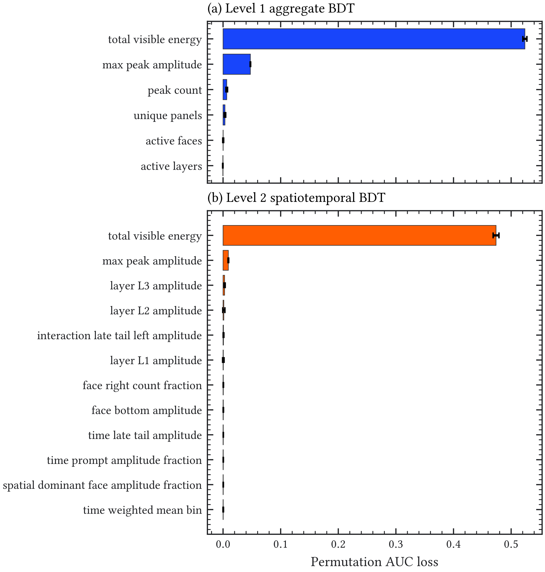
The level-1 feature vector contains total reconstructed veto-energy proxy, peak count, unique semantic panel count, active face count, active layer count, and maximum peak amplitude. The full level-2 vector contains 164 observables after adding per-window count and amplitude summaries, face and layer occupancies and entropies, opposite-face activity, and position–time cells. Both models use a HistGradientBoostingClassifier with 220 boosting iterations, learning rate 0.045, at most 12 leaves, minimum leaf size 30, regularization 0.10, balanced class weights, and fixed random seed 20260829. No Micromegas observable is used.
At the nominal 90% operating point, level 1 accepts 24,798 of 27,529 held-out calibration events and rejects 3377 of 4035 held-out neutron events. The full level-2 model accepts 24,851 calibration events and rejects 3396 neutron events. The paired 3000-replicate bootstrap gives a level-2 minus level-1 rejection difference of 0.47 percentage points, with a central 90% interval of 0.07–0.82 percentage points; the AUC difference is consistent with zero. Removing total reconstructed energy from the full model reduces the rejection to 3190 of 4035, or , while retaining held-out control acceptance. This ablation demonstrates discriminating timing and segmentation information within the overlaid sample, together with the dominant role of the reconstructed-energy response.
A.4.1.1 Recorded-window boundary check
The aligned neutron input contains 385 peaks outside bins 0–511, distributed over 153 of the 20,274 events; 34 affected events belong to the 4035-event held-out partition. Clipping these peaks to bin 0 creates recorded activity where the model should instead reject an unrecorded peak. The revised feature constructors round to a sample and reject out-of-range or non-finite times before computing peak counts, amplitudes, and spatial or timing features. Historical model files and thresholds are retained, allowing a bounded comparison with no retraining.
| Frozen model | Nominal acceptance | Historical tags | Boundary-check tags |
|---|---|---|---|
| Level 1 | 3377 | 3377 | |
| Level 1 | 3328 | 3328 | |
| Level 2 without total energy | 3190 | 3170 | |
| Level 2 without total energy | 2985 | 2962 |
The full level-2 model also retains its historical tag count in this limited comparison, whereas the model without total energy loses 20 and 23 tags at the two operating points. These changes quantify the local feature defect, not the full acquisition-response uncertainty. The empirical bin alignment, absent simulated support above , and unavailable calibrated energy per peak require a waveform replay with a common trigger convention before producing replacement efficiency estimates. The revised training and dataset-building paths reject an affected sample when they would combine window-corrected peaks with the old unwindowed energy scalar.
A.4.1.2 Capture-delay feature construction and checks
The capture-specific diagnostic is identified by capture-delay-signature-20260829-r1. It reuses the hierarchy’s frozen run partition and classifier hyperparameters, but replaces the generic disjoint timing windows with aligned timing coordinates defined by Equation (1.1). The prompt and capture-like intervals are and , respectively. These intervals were fixed before the held-out comparison from the empirical timing convention and the independent HENSA capture-history study.
The seven timing coordinates are two peak-presence indicators, a prompt–delayed coincidence indicator, the time of the first delayed peak, the gap from the last prompt peak to the first delayed peak, and the delayed amplitude-weighted time mean and standard deviation. The complete 18-variable signature adds prompt and delayed peak counts and amplitude sums, prompt and delayed panel multiplicities, delayed face and layer multiplicities, delayed count and amplitude fractions, and the number of panels active after but not during the prompt interval. All quantities are constructed after mapping simulation and prototype channels independently into the common semantic panel coordinate. Missing first-peak and gap coordinates are represented by zero only in conjunction with their explicit presence indicators.
The 159,728-event classifier sample contains 139,454 experimental calibration events and 20,274 simulated HENSA events with independently sampled calibration activity overlaid. All peak channels map successfully, all engineered quantities are finite, and the original six-variable level-1 AUC and operating point are reproduced exactly by the independent script. No Geant4 capture label, Micromegas observable, run identifier, or overlay index enters the classifier. The truth sample is used only to verify that the physical cadmium-capture distribution supports the chosen interval. Its 55,581-record denominator is explicitly restricted to ; is the cumulative fraction up to , while the actual – truth-window fraction is .
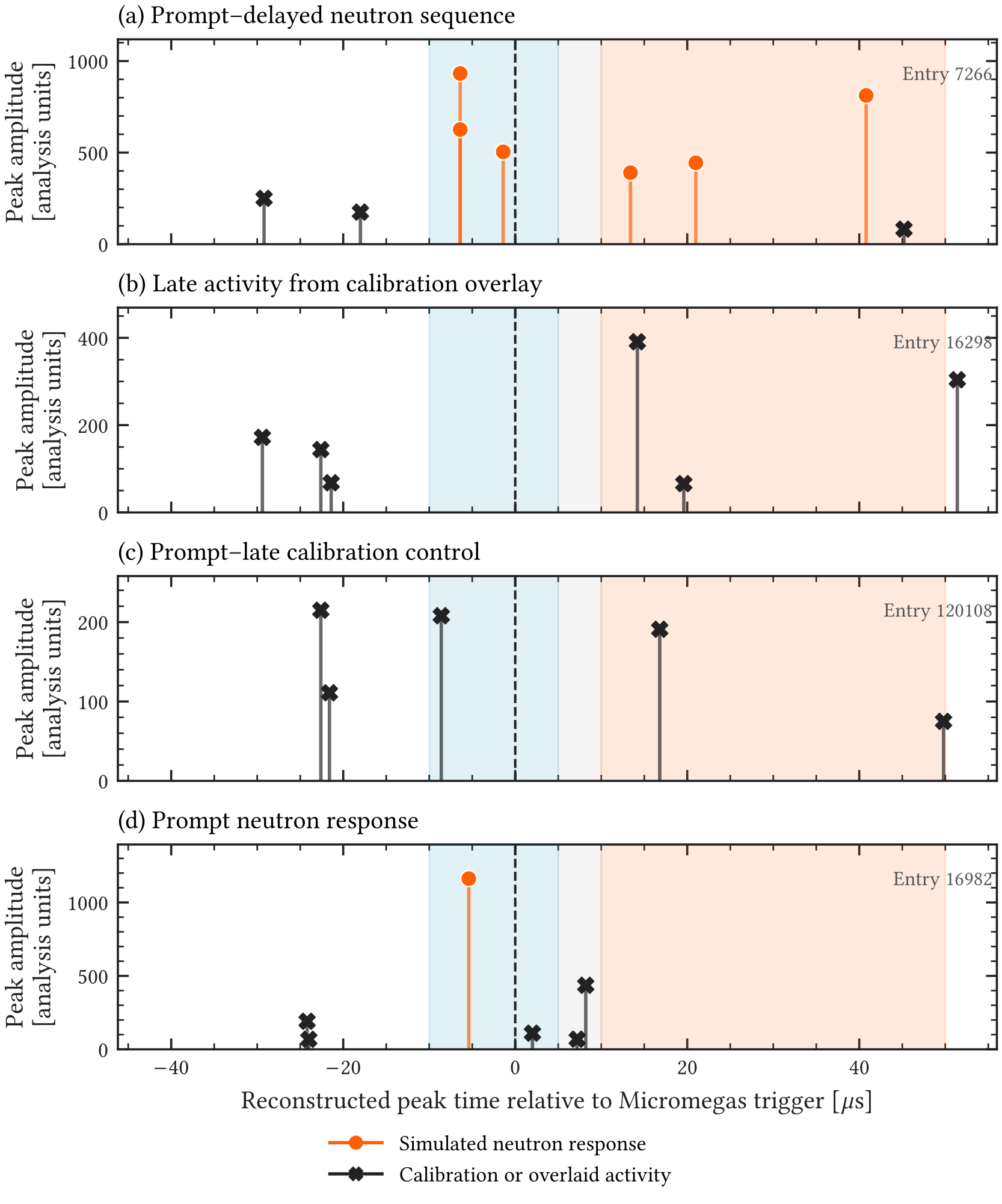
At nominal 90% control acceptance, the trigger-relative coordinate-only model rejects 2011 of 4035 held-out neutrons, the full capture-signature model rejects 2991, and the level-1-plus-signature model rejects 3397. The corresponding held-out control acceptances are , , and , respectively; level 1 alone accepts and rejects 3377 neutrons. For the combined model, the paired 3000-replicate bootstrap gives a rejection difference of percentage points with a central 90% interval of to points. Its AUC difference has median and interval to , compatible with zero.
The independent event-mixed test uses 250 circular time shifts for each of 879 neutron events. The complete peak train of a randomly selected neutron event is shifted as a unit within , preserving its energy, multiplicity, and spatial structure while removing its causal alignment with the trigger. The central 90% ranges of time-scrambled control acceptance are – for a late peak alone, – for prompt plus late activity, – after requiring two delayed groups, and – after the delayed-energy requirement. Because this null model is constructed from neutron peak trains, its acceptance is not a measured experimental random-coincidence probability and need not be an upper bound on that probability.
Among the 2659 selected events containing at least one truth-level cadmium capture, 644 have no reconstructed veto peak, a conditional fraction of . The same 644 events are of the complete 2706-event selected sample.
The validation script checks the declared time-coordinate definition, complete event merge, channel-map closure, exact level-1 reproduction, monotonic truth-capture retention, and the predeclared behavior of the event-mixed signatures. These are reproducibility checks on the historical capture-specific ablation. Level 1 remains its reference selector because the combined-model five-run control-acceptance minimum is , compared with for level 1.
A.4.1.3 Level-3 spatiotemporal neural model
The frozen level-3 representation contains only reconstructed veto peaks. For every event, a compact sparse list is expanded per minibatch into a tensor on the common prototype–simulation panel support. The first channel is the summed peak amplitude in each panel–time cell after a transformation and training-partition normalization; the second is the peak occupancy. The simulation-only Top_L1_N4 panel is excluded because it has no prototype counterpart. The six level-1 aggregates form a separately normalized optional branch. Run, subrun, event, raw-channel, overlay, TPC, and Geant4-truth quantities are retained only as audit metadata and never enter the network.
The shared temporal encoder applies three one-dimensional convolutional stages with kernel sizes 9, 7, and 5 and stride 2 to every panel. Learned embeddings identify the panel face, layer, and within-face number. Two relational graph blocks then propagate messages through three fixed adjacency matrices: neighboring panels on the same face and layer, corresponding panels in adjacent layers, and corresponding panels on opposite faces. An attention-weighted sum over the remaining panel–time tokens feeds the final classifier. The predeclared hybrid concatenates this representation with a 24-dimensional encoding of the six level-1 aggregates and contains 53,330 trainable parameters. Training used 20 epochs of AdamW optimization, binary cross entropy, a batch size of 256, and 3% random panel dropout on a CERN SWAN CUDA session.
Four variants were trained with the same run-disjoint partition and frozen thresholds. At nominal 90% control acceptance, the scalar multilayer perceptron rejects 83.82% of held-out neutrons, the tensor-only temporal model 71.15%, the tensor-plus-graph model 72.64%, and the hybrid 84.11%. The graph therefore recovers 1.49 percentage points relative to temporal convolution alone, but the tensor branch still requires the aggregate branch to match the boosted-tree baseline. Relative to level 1, the hybrid rejects 17 additional held-out neutrons net: 38 are rejected only by the hybrid and 21 only by the BDT. The paired-bootstrap rejection difference is percentage points with a central 90% interval of to percentage points; the AUC difference, , is compatible with zero.
The frozen-threshold perturbation audit shifts all peaks by and bins, rescales their amplitudes by 0.9 and 1.1, and masks one representative panel in every face–layer cell. Across these tests, neutron rejection changes by at most to percentage points for amplitude scaling, to points for time shifts, and to points for panel masks. The corresponding control acceptance can shift by as much as points. The five-run acceptance range is 83.38–90.61% at the nominal 90% threshold; the low value occurs in training run 1339 and demonstrates that the run dependence identified at level 2 is not removed by the neural representation.
For the independent conservative-reference application, the raw veto vectors of all 249 candidates were extracted directly from their archived AnalysisTree entries and checked against the requested event identifiers. The three causal-history activation events were excluded, leaving 246 prompt/non-delayed events. Two hundred independently seeded empirical-noise overlays were evaluated for every candidate. At the nominal 90% level-1 threshold the mean survivor count is 21.8, with a central 90% overlay range of 19–25; the first reproducible draw leaves 22 events. The corresponding full-model mean is 20.6, with a range of 18–23. The level-3 hybrid mean is 21.0, with a range of 18–24, and its first reproducible draw leaves 20 candidates. All candidate-level scores, overlay calibration indices, model files, feature manifests, and causal labels are retained in outputs/veto-analysis/veto-bdt-hierarchy-20260829-r1.
The neural dataset, CUDA checkpoints, held-out scores, robustness audit, run-stability table, and candidate overlays are retained in outputs/veto-analysis/veto-level3-20260829-r1.
This boosted-tree hierarchy is distinct from the richer experimental control-population score described below. The level-3 result is not used to renormalize the prompt background because it does not satisfy the predeclared material-improvement and run-stability gates.
A.5 Calibration-controlled late-window population
The exploratory prototype reanalysis asks which background events resemble late-window HENSA-neutron templates more than calibration or prompt-muon controls. It is not used as a neutron-fraction measurement. The term selected control event below means only that the event passes the frozen score requirement.
A.5.1 Input products and preprocessing
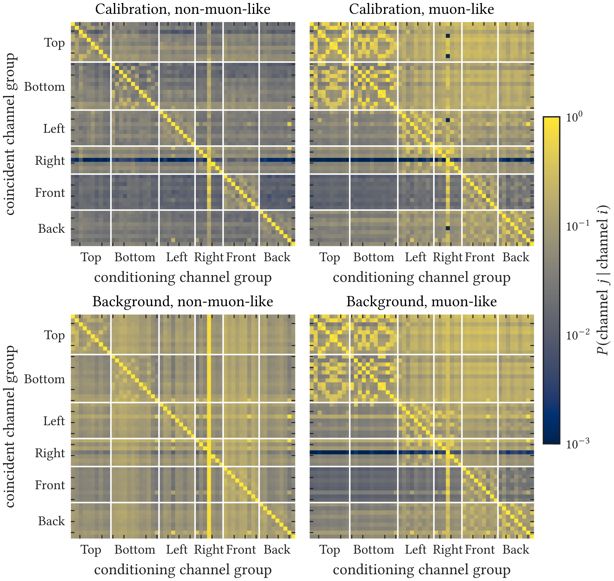
Two experimental background products are used for different diagnostics. The merged paper-analysis file contains 995,271 entries and supports direct vector-branch and channel-correlation studies. The flattened score input contains 777,752 feature-complete events after the preprocessing used by the classification workflow. The calibration score input contains 139,454 events. The 995,271- and 777,752-event denominators are not interchangeable.
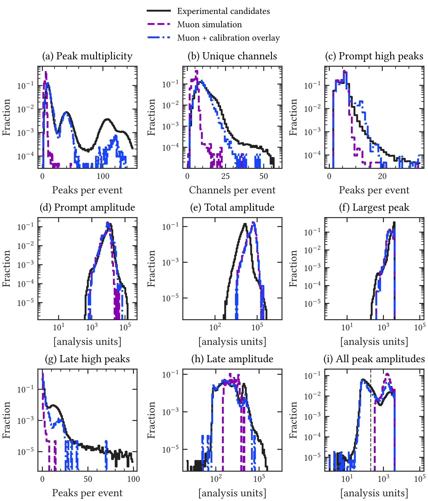
The simulation templates contain 21,569 analyzed muon entries and 20,274 analyzed neutron entries after merging the waveform-level production outputs. Calibration-triggered veto peak trains are concatenated with each simulated event, retaining correlations among the measured peaks in a donor event. Because this operation follows peak finding, it does not model merged pulses, baseline changes, threshold migration, or saturation when simulated and measured pulses overlap. REST peak times are mapped to the experimental bin convention through
(A.1)
The prompt alignment selects muon entries in the unoverlaid template and entries in the merged experimental background product. The separate flat score input has a prompt-tag fraction after its own preprocessing.
A.5.2 Score definition
Three time regions are defined in the mapped bin coordinate of Equation (A.1): the prompt region , the near-capture region , and the inclusive late region . The implementation historically calls the near-capture region the “neutron window.” The late region overlaps it and is an in-waveform observable; neither region is the long-lived delayed-activation channel defined from event history in Section 6.7. For non-negative energy-like inputs, the transformation is . The event vector is
(A.2)
where is clipped at 59 channels and the near/late multiplicities count peaks above 200 analysis units. The one-dimensional histograms use 53 uniform edges over , unit-width edges over , 55 uniform edges over , unit-width edges over , unit-width edges over , and 66 uniform edges over , in the order of Equation (A.2). Each class likelihood is the product of the six separately normalized one-dimensional histograms after adding to every bin,
(A.3)
The resulting naive product ignores correlations, including the overlap between the near and late windows, and is used only as an ordering statistic. The score is
(A.4)
Prompt-muon events are removed with for peaks above 200 analysis units in bins . Events with at least 100 veto peaks or 50 unique veto channels are excluded as burst-like. The frozen control threshold is the upper tail of the clean calibration score distribution,
(A.5)
The exact value is reported for reproducibility and should be read as the 99th calibration percentile, not as a universal physical threshold.
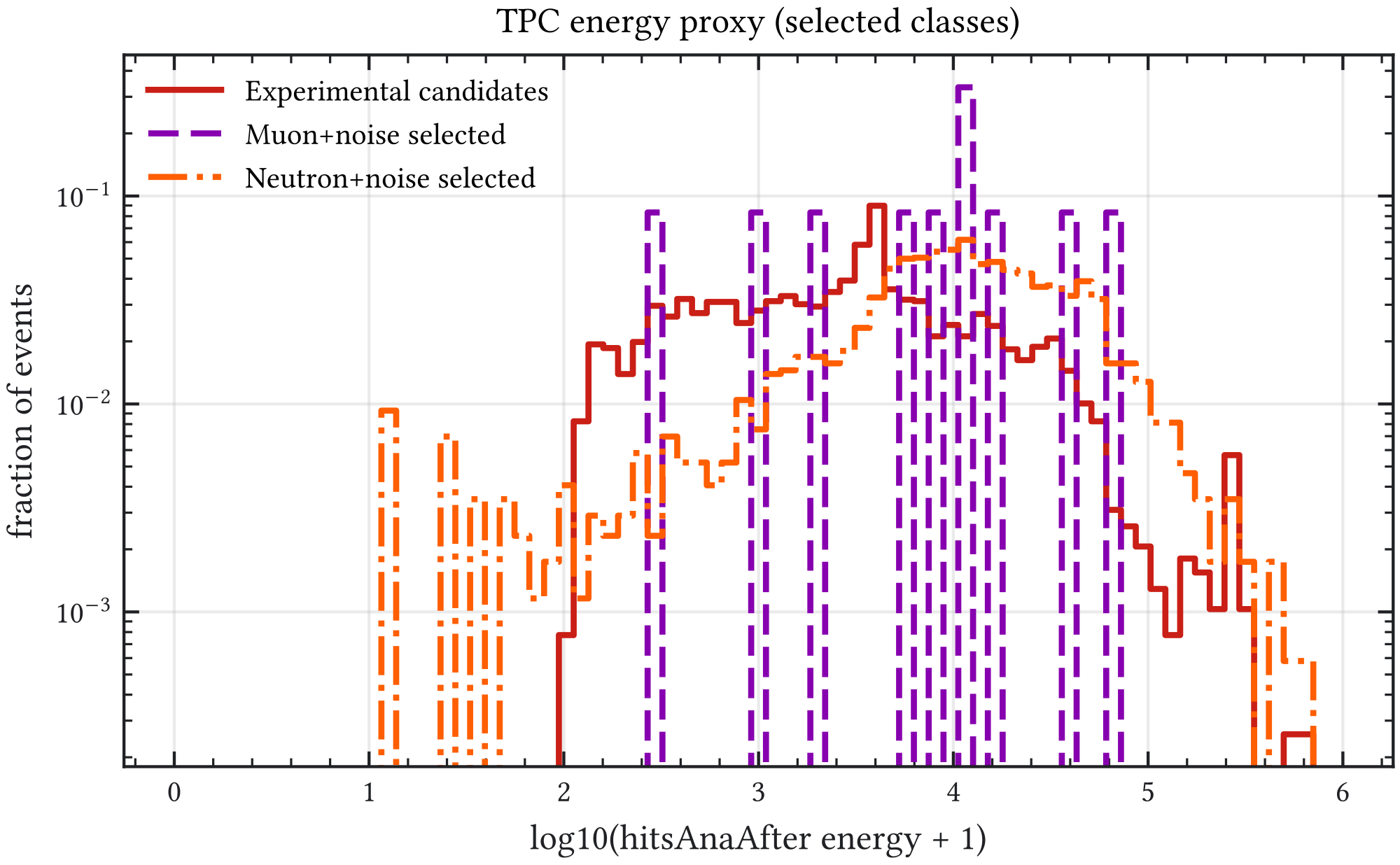
The score distributions and population-level selection counts are reported in Figure 1.22 and Table 1.7 of Section 5. They are kept in the main chapter because they are the quantitative result of the control-population study; the definitions above provide its reproducible construction.
A.5.3 Template mismatch and interpretation
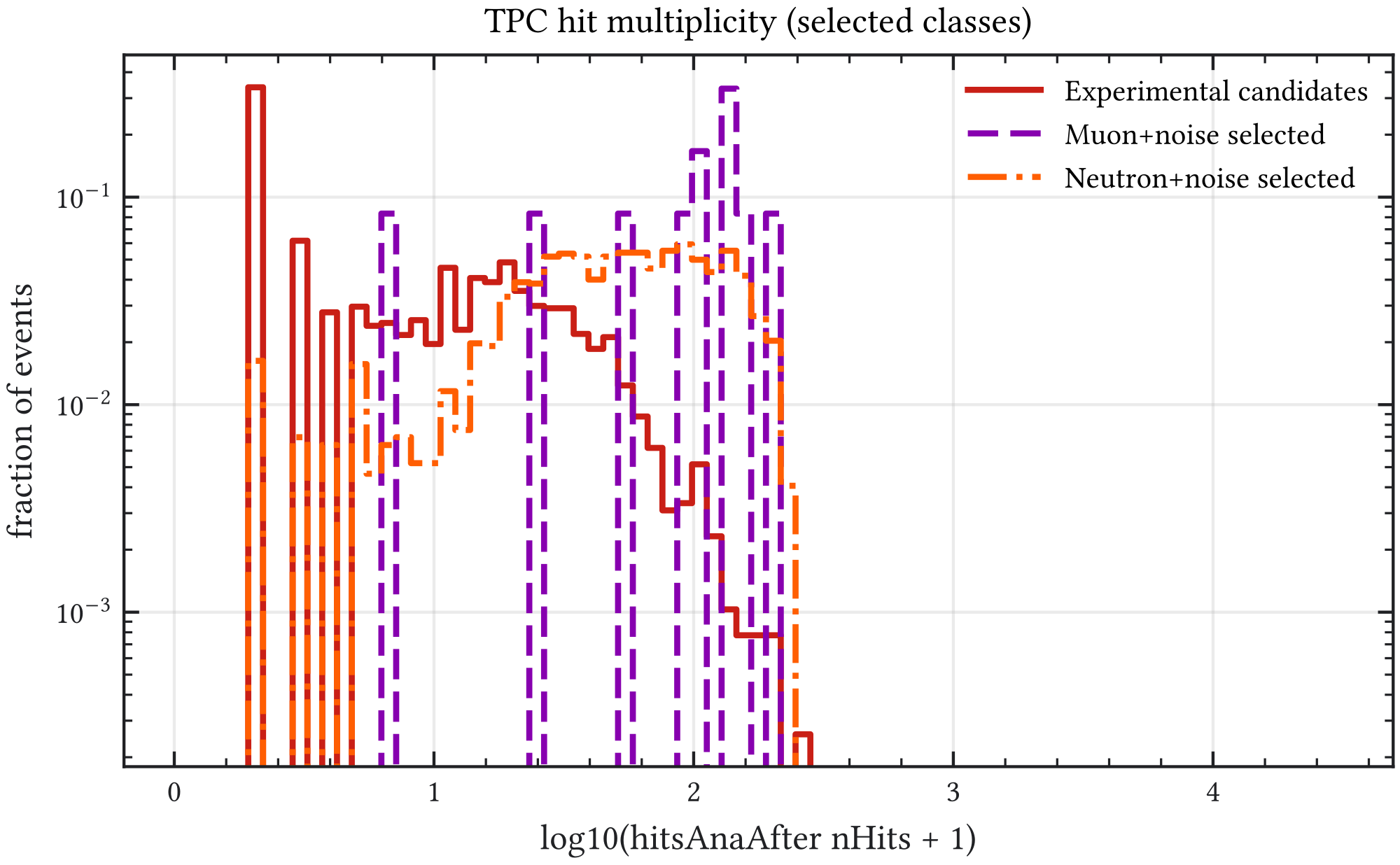
The score selects experimental events, or of the full flat input and of the clean prompt-suppressed subset. The selection suppresses the prompt-muon population and, by construction, accepts only the upper score tail of the calibration control. It does not establish that the residual background events have a non-accidental origin: the Micromegas energy enters the score, and the control and background samples differ in energy distribution, operating conditions, and acquisition history. The current HENSA template also fails to reproduce the selected population quantitatively.
| Median observable | Selected data | Selected neutron+noise |
|---|---|---|
| Veto peaks | 47 | 9 |
| Unique veto channels | 12 | 8 |
| Total veto-energy proxy | 11249 | 13513 |
| Near-capture-window peak count | 1 | 1 |
| Late-window peak count | 7 | 4 |
| Late-window energy proxy | 6822 | 2707 |
| Micromegas energy observable | 3025 | 10566 |
| Micromegas hit multiplicity | 6 | 51 |
| topology variable | 2.31 | 14.19 |
| topology variable | 2.70 | 7.59 |
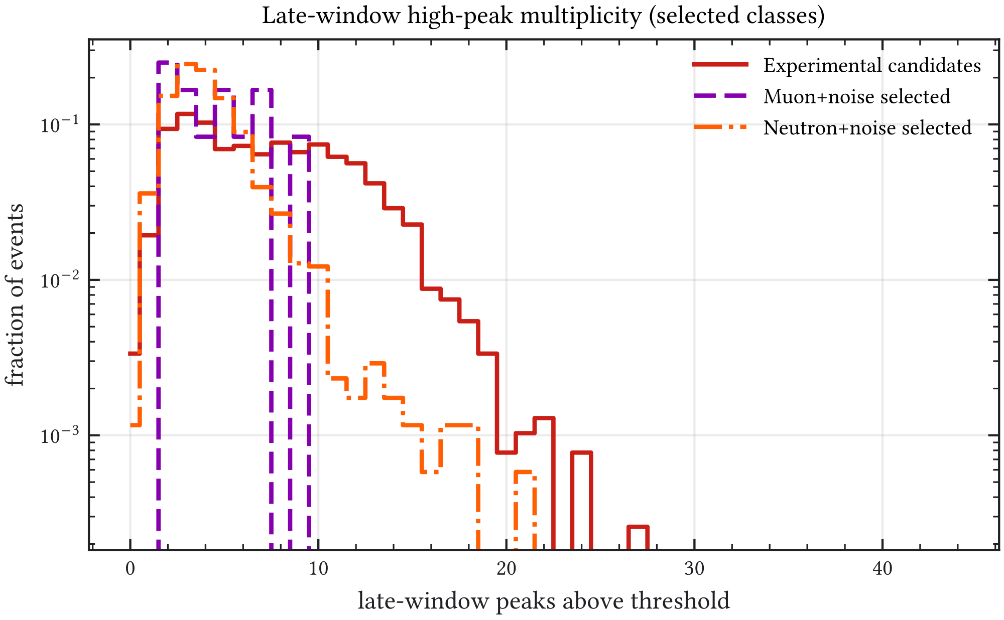
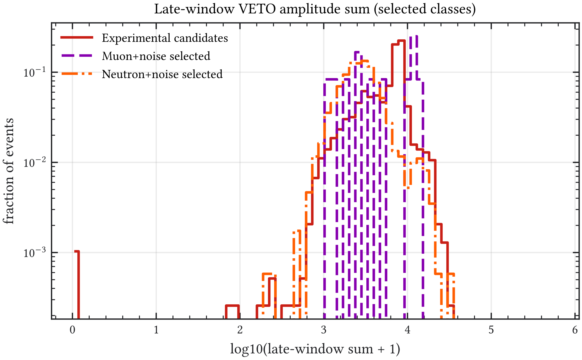
Candidate rasters and Micromegas-topology projections are given in Appendix Section A.10. The existing samples support a more direct control test: match calibration and background events by run conditions and Micromegas energy, construct time-shifted accidental controls, and repeat the comparison with a veto-only score on a held-out run. Pseudo-data mixtures can then test how much neutron-like activity would be identifiable under the observed template mismatch. A physical neutron-fraction measurement would additionally require independently calibrated neutron-response templates and competing-background controls. The selected count is therefore retained as a control-population observable.
A.6 Supplementary veto simulation campaign metadata
The main veto-system chapter uses compact labels for the simulation campaigns in order to keep the design argument readable. The table below retains the source, response, and timing conventions needed to distinguish historical design scans, selected HENSA design-study productions, and experimental prototype validation.
| Study | Primary sample | Geometry / response level | Timing convention | Statistical / reproducibility note |
|---|---|---|---|---|
| Inclination scan | Guan muons and HENSA outdoor neutrons in their detector-relevant energy ranges | Full shielded detector; comparison of processed TPC response | Not applicable | Each source is normalized independently to the horizontal geometry; the neutron response spans – and the muon response –. |
| Lead and passive-neutron scans | CRY mixed secondaries or neutrons, as stated in each study | Parameterized shielding geometries; post-analysis TPC background rate | Not applicable | Common transport and analysis settings kept fixed within each geometry scan so that only the shielding layout changes. |
| Simplified material scans | High-energy neutron samples on slab and early multilayer layouts | Deposited or Birks-quenched visible energy before the final readout chain | Not applicable | Comparative material-ordering diagnostics; not final reconstructed efficiencies. |
| Selected HENSA layer scan | HENSA outdoor neutrons in one- through four-layer Cd layouts and three-layer material variants | Selected 59-panel design-study response chain with quenching, attenuation, 200 ns veto sampling, 1014 ns shaping, and peak finding | Production REST alignment uses TRIG_DELAY_VETO | Every processed AnalysisTree entry is exported; no conservative-reference Micromegas selection is applied. |
| Experimental validation | Surface IAXO-D0 prototype data set (52.1 days) | Commissioned 57-panel implementation analyzed with waveform observables; current reprocessing uses 200 ns veto sampling | Published hardware record of approximately 100 s with the Micromegas trigger 30 s after its start | The REST alignment parameter used in reprocessing is distinct from the published hardware trigger position. Event counts, central levels, and calibration efficiencies follow the publication; exact 90% Poisson intervals are recomputed from the counts. |
A.7 Supplementary active-veto design diagnostics
The main text uses a simplified representative sandwich comparison to motivate the active-material choice. The full ordering scan and the quenching diagnostic are retained here because they document that the qualitative conclusion is stable across the scanned material orderings.
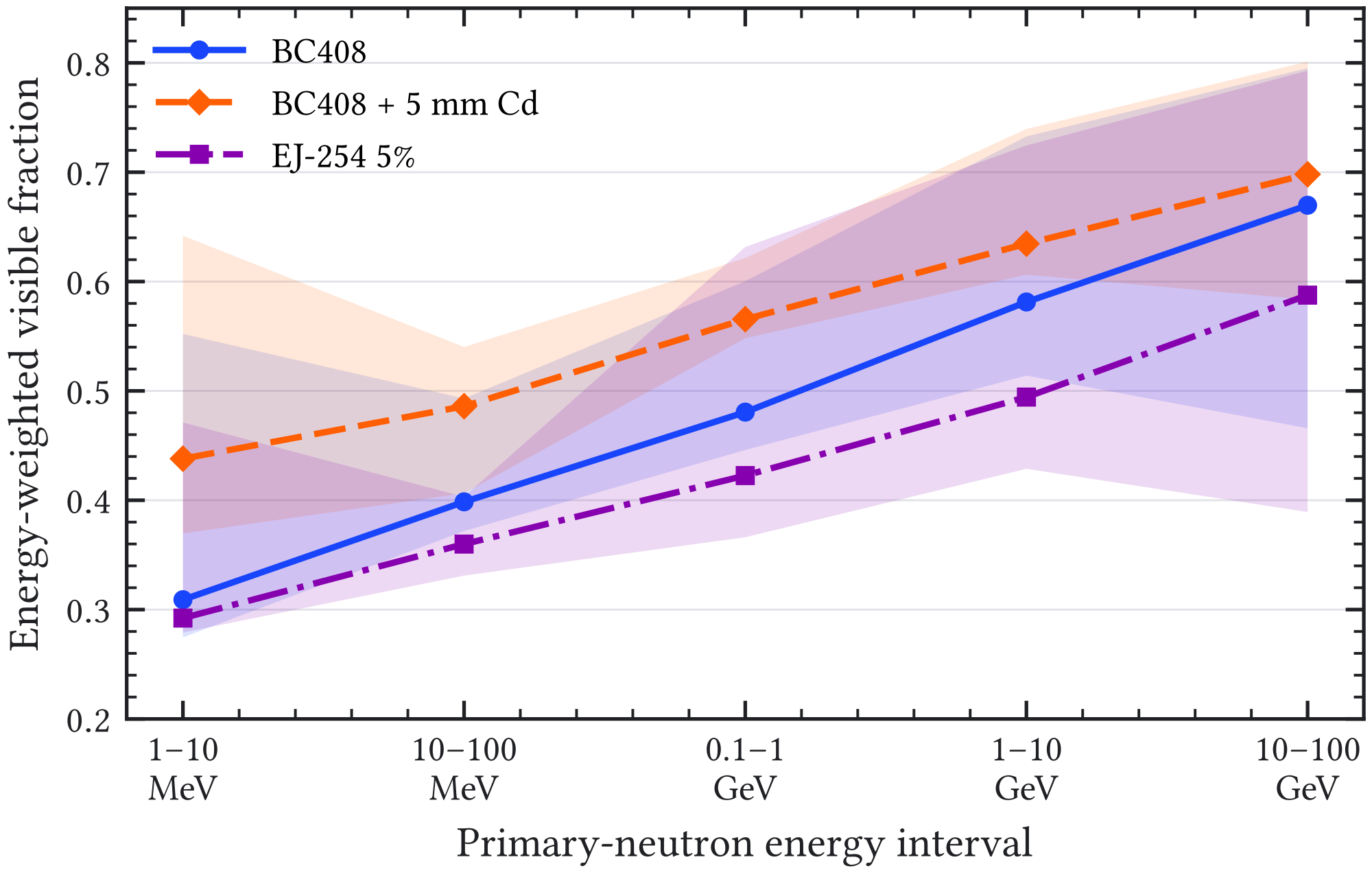
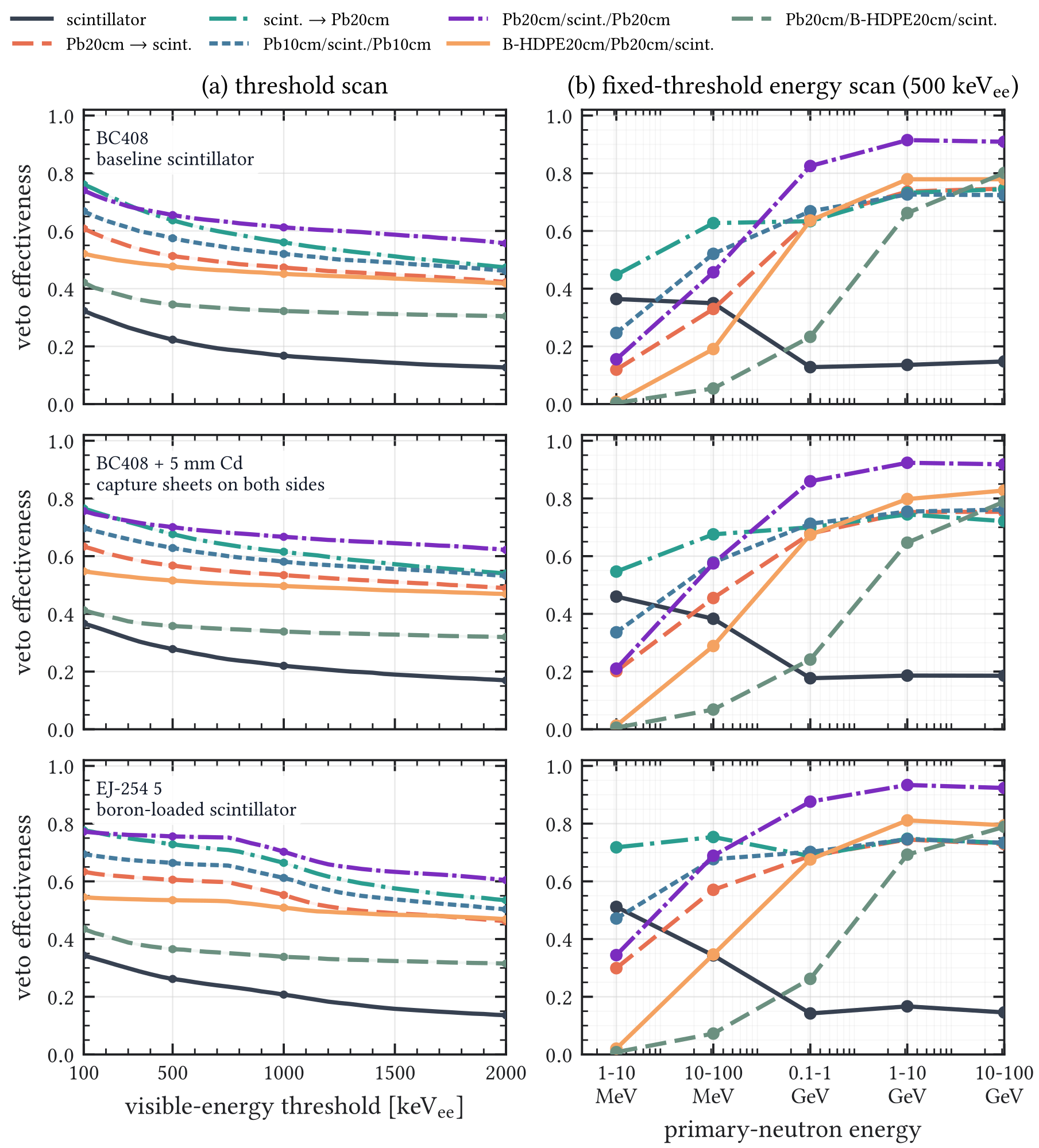
A.8 Supplementary HENSA veto layer-scan diagnostics
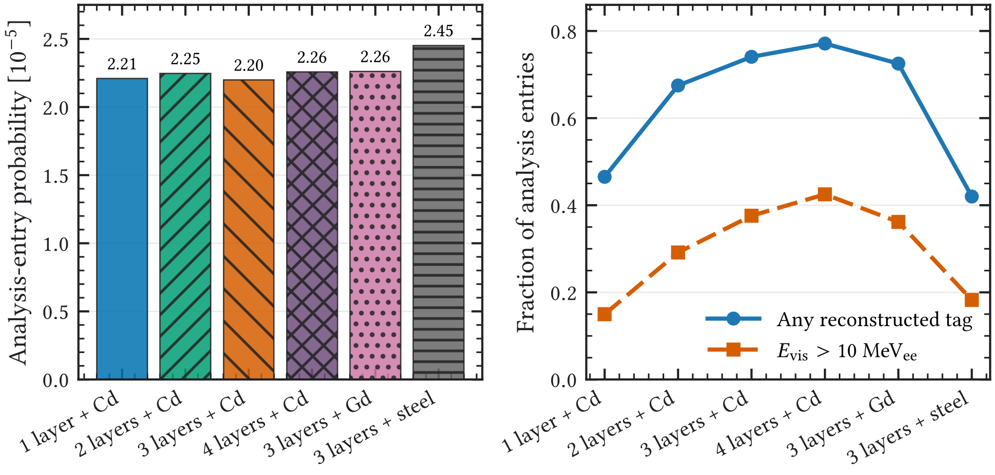
The main veto-system chapter uses a compact layer-design figure that combines threshold response and conditional tagging. The diagnostics below retain the generated-primary exposure recovered from the NAF job logs and the corresponding processed-analysis-entry probability. This replaces the earlier job-hour normalization, which measured computational throughput rather than physical exposure.
| Configuration | Files | Primaries | Entry prob. | Any tag | Rej. 10 MeV |
|---|---|---|---|---|---|
| 1 layer + Cd | 300 | 0.465 | 0.150 | ||
| 2 layers + Cd | 300 | 0.675 | 0.292 | ||
| 3 layers + Cd | 300 | 0.741 | 0.376 | ||
| 4 layers + Cd | 300 | 0.771 | 0.425 | ||
| 3 layers + Gd | 230 | 0.725 | 0.362 | ||
| 3 layers + steel | 230 | 0.420 | 0.183 |
AnalysisTree entries exported without an additional Micromegas selection, divided by the generated-primary count recovered from all corresponding NAF job logs. “Any tag” and “Rej. 10 MeV” are conditional on those analysis entries. All 1–4-layer cadmium configurations have entry probabilities near ; the layer-dependent gain is in reconstructed veto tagging.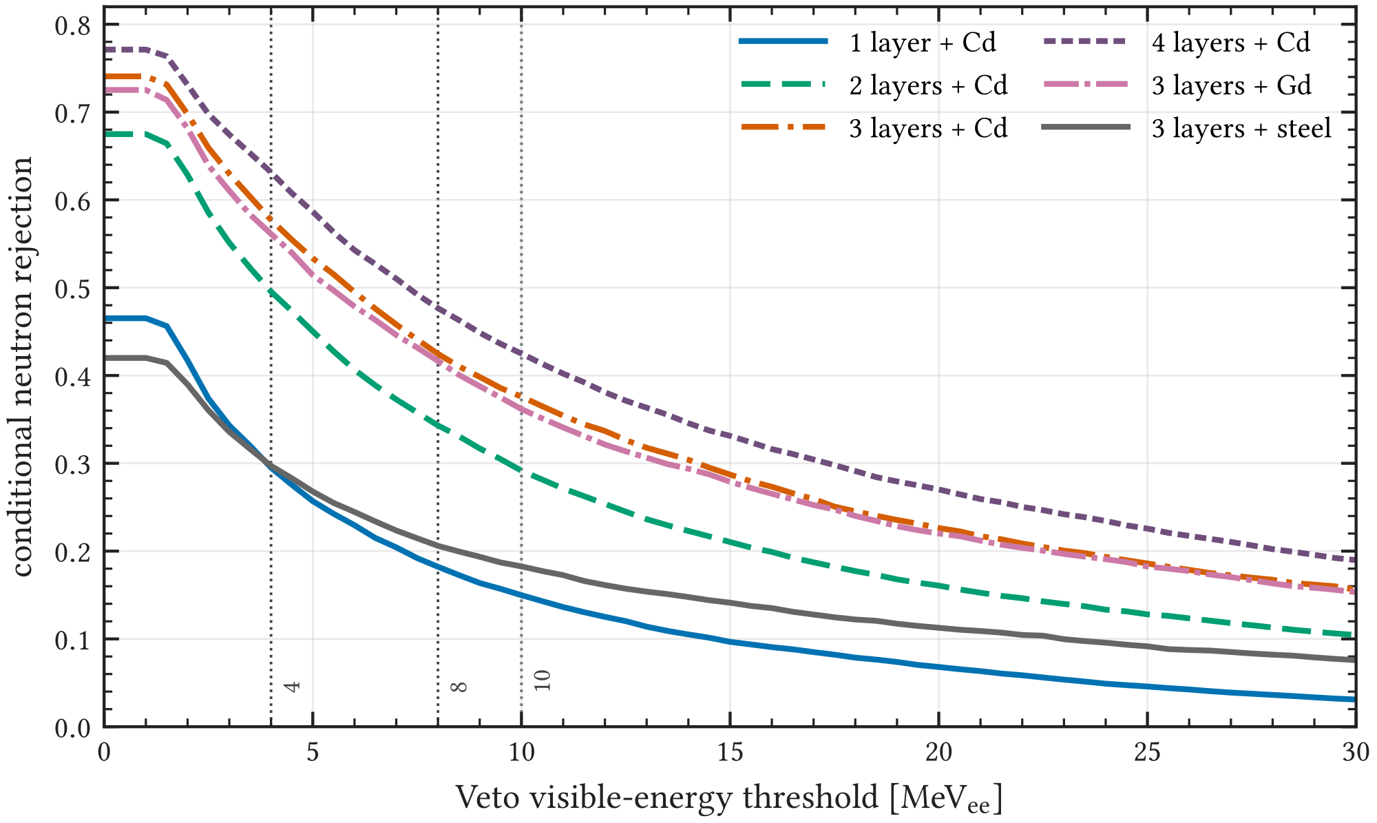
A.9 Supplementary neutron-tagging diagnostics
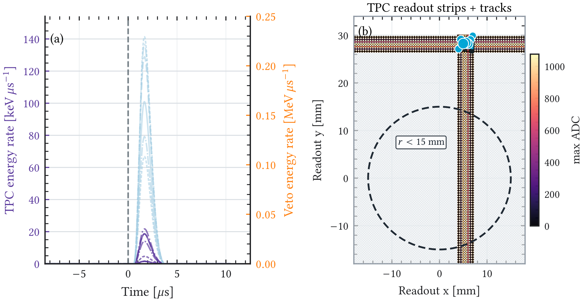
The capture-material, timing, and truth-to-reconstruction summary is presented in Figure 1.8 of Section 5 because it is part of the central veto-mechanism result. The event display below retains a selection-level diagnostic that is not needed for the design argument.
A.10 Supplementary late-window control diagnostics
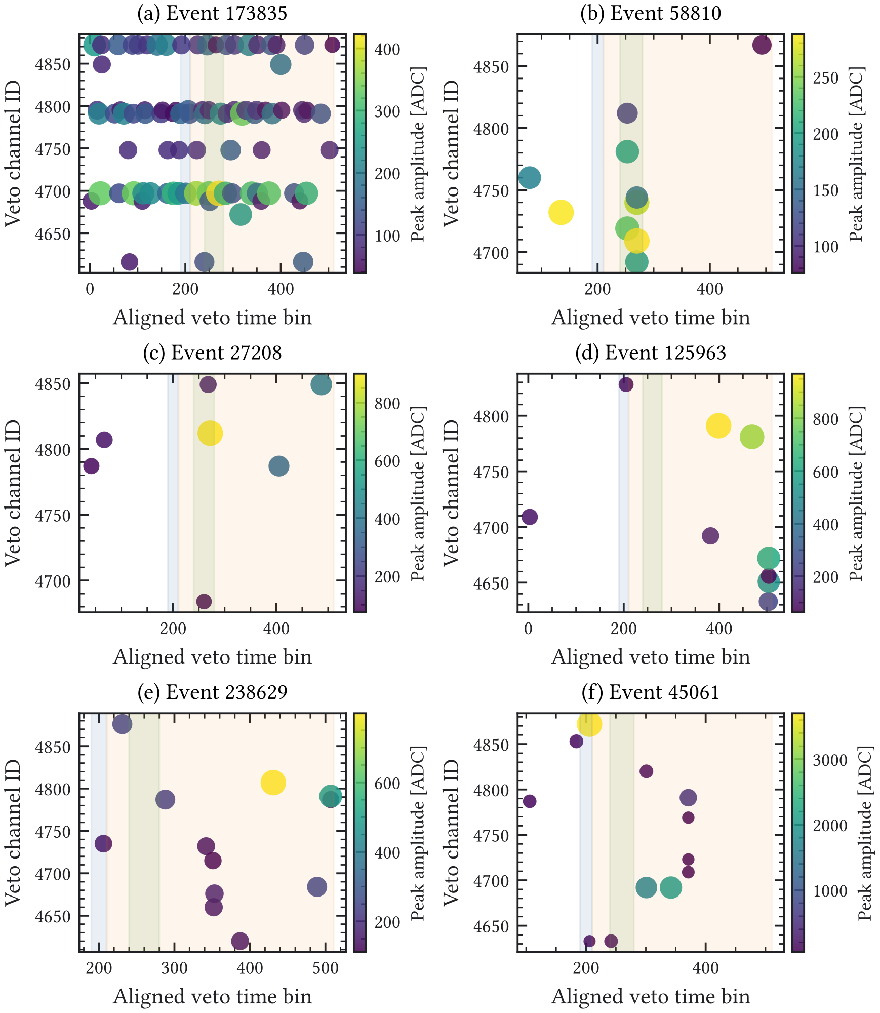
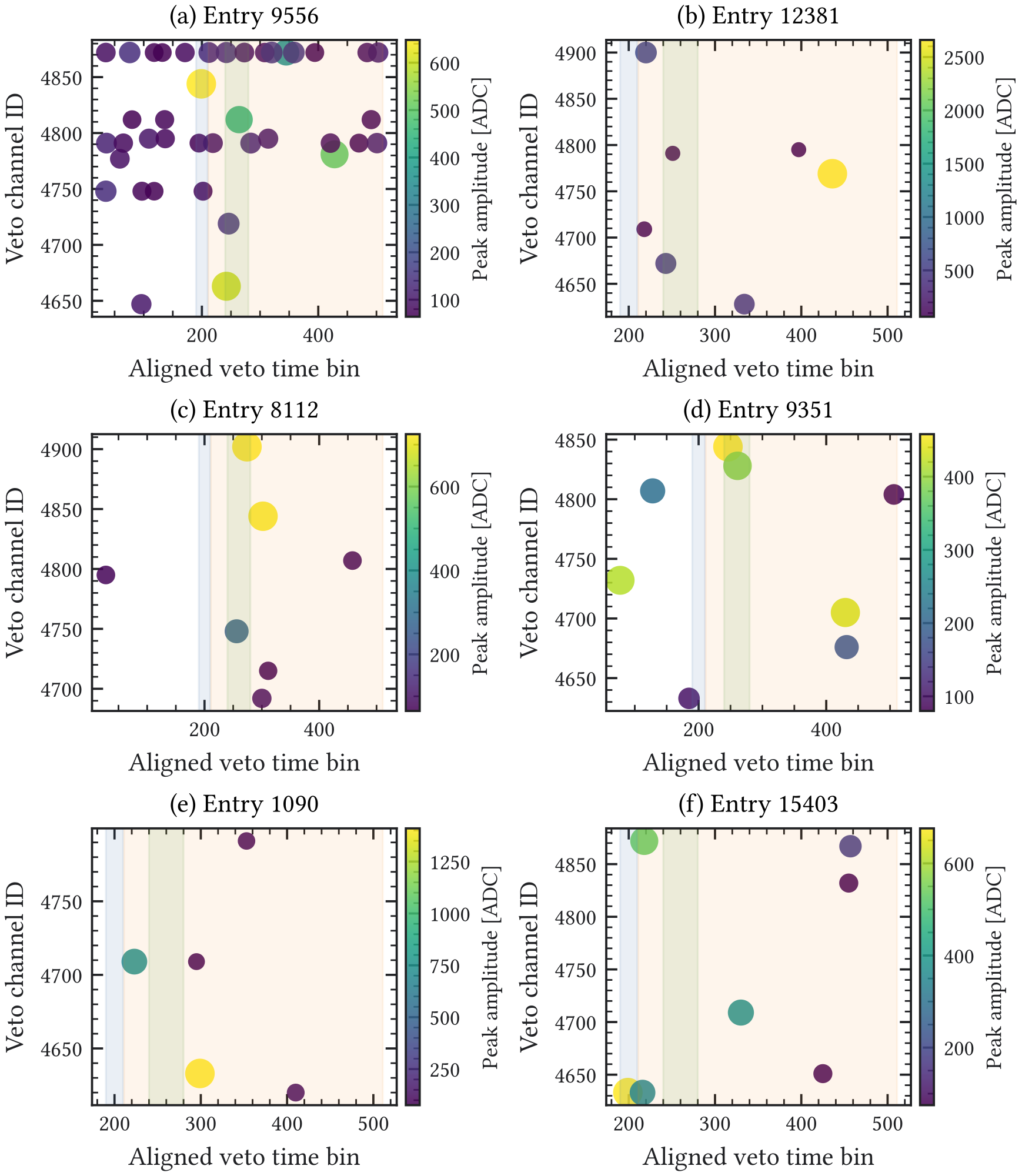
The score definition and its population-level interpretation are given in Section A.5. The event-raster and Micromegas-topology projections below document the residual differences between the selected experimental control population and the selected neutron+noise simulation.
A.11 Supplementary passive-shielding scans
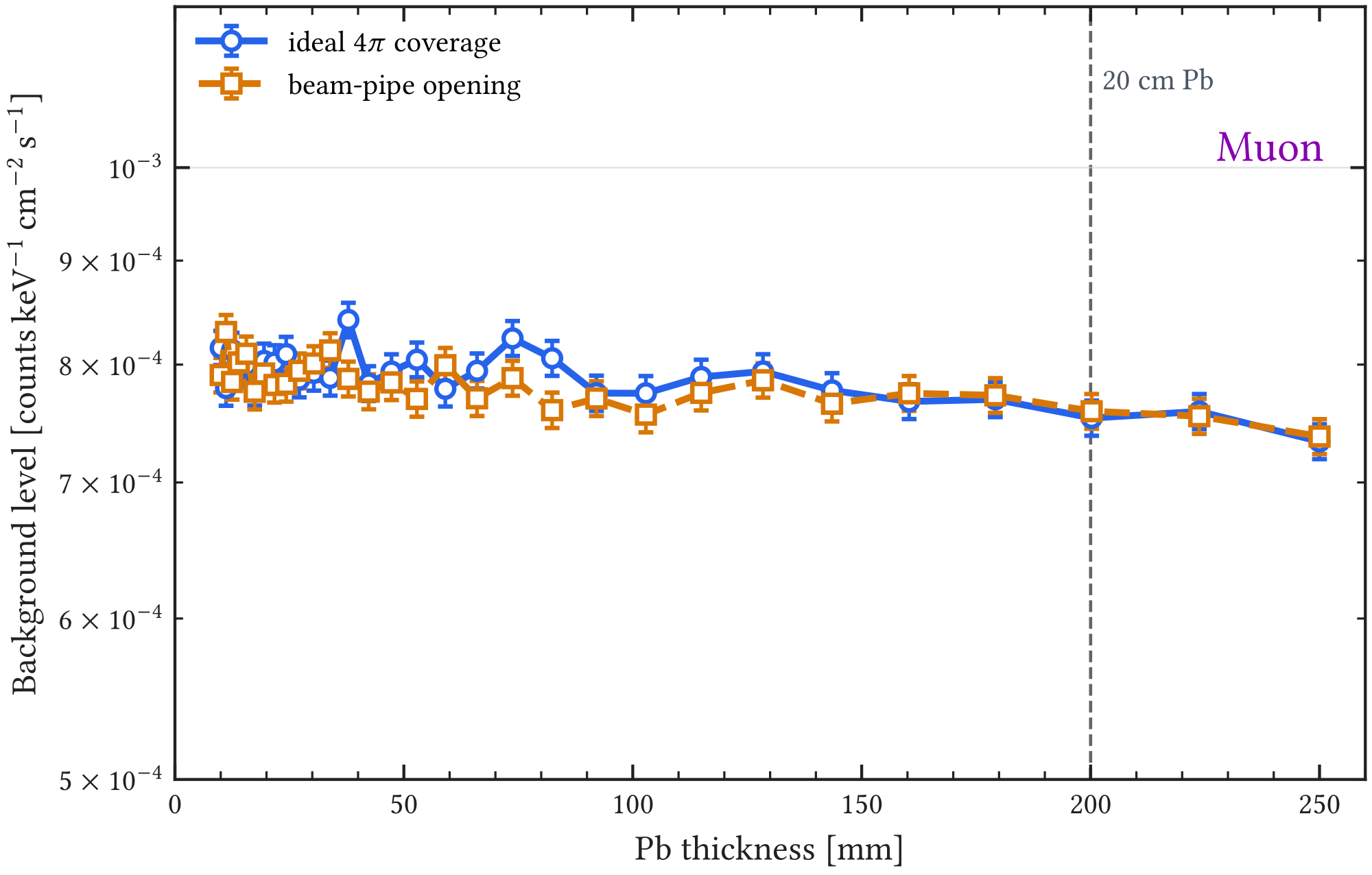
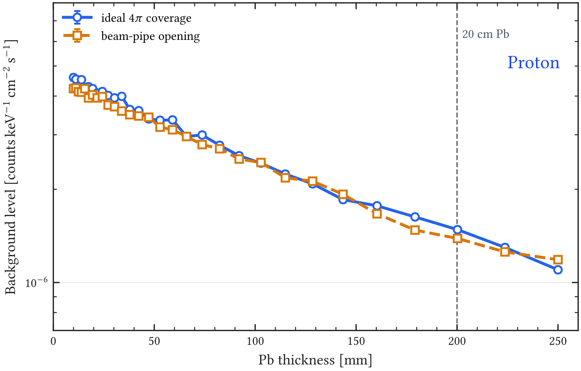
The main shielding and veto chapter uses a compact photon/neutron summary of the lead-thickness scan because those two components determine the passive-shielding design decision. The full per-particle scans are retained here as simulation provenance and as checks that the other cosmic-ray-induced components do not change the conclusion.
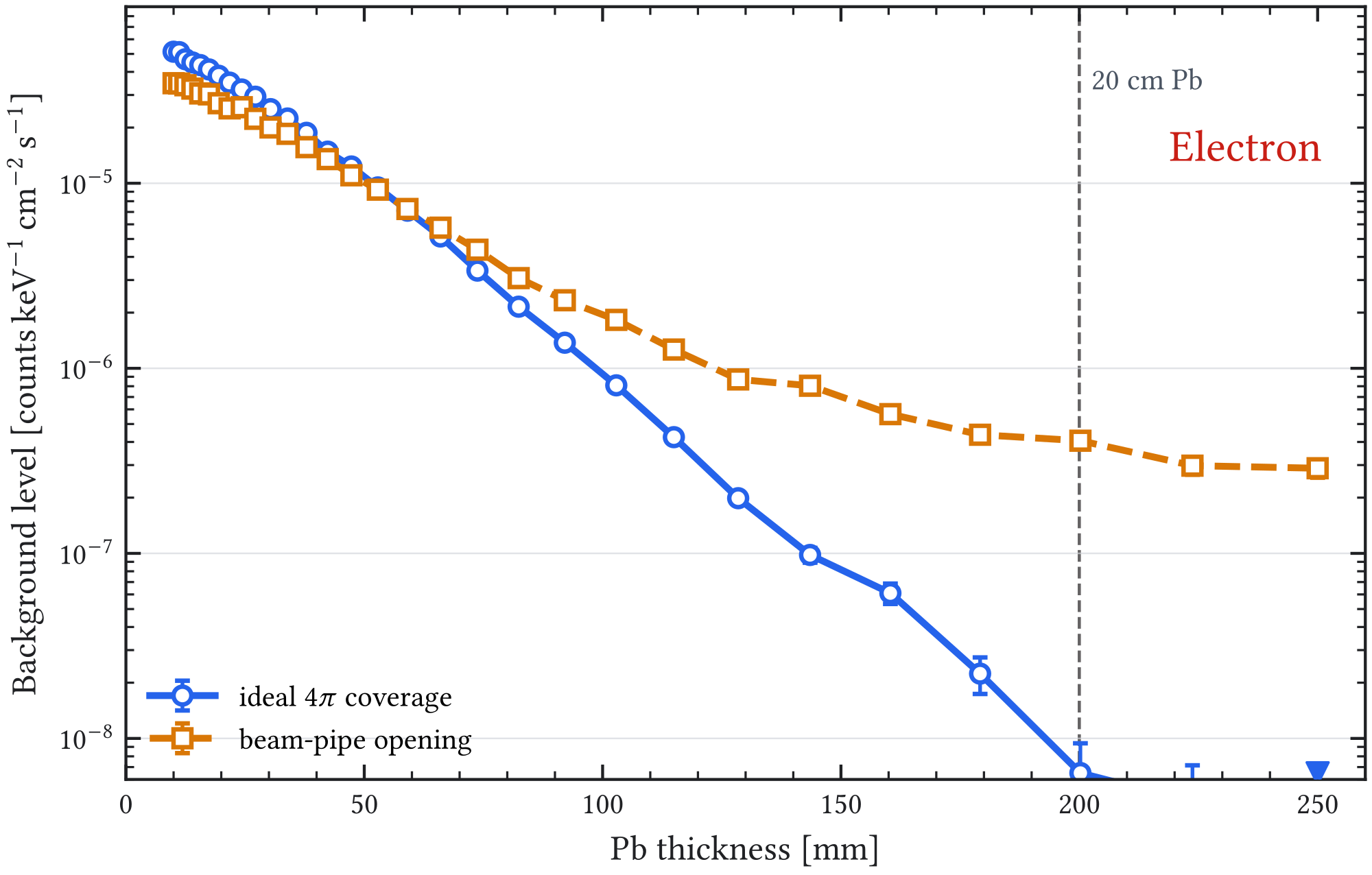
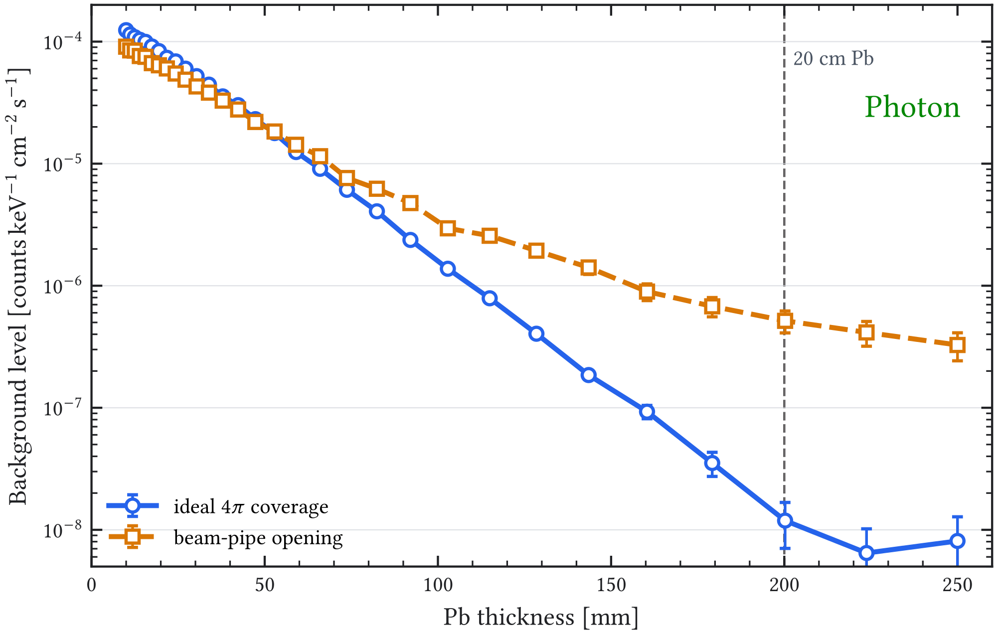
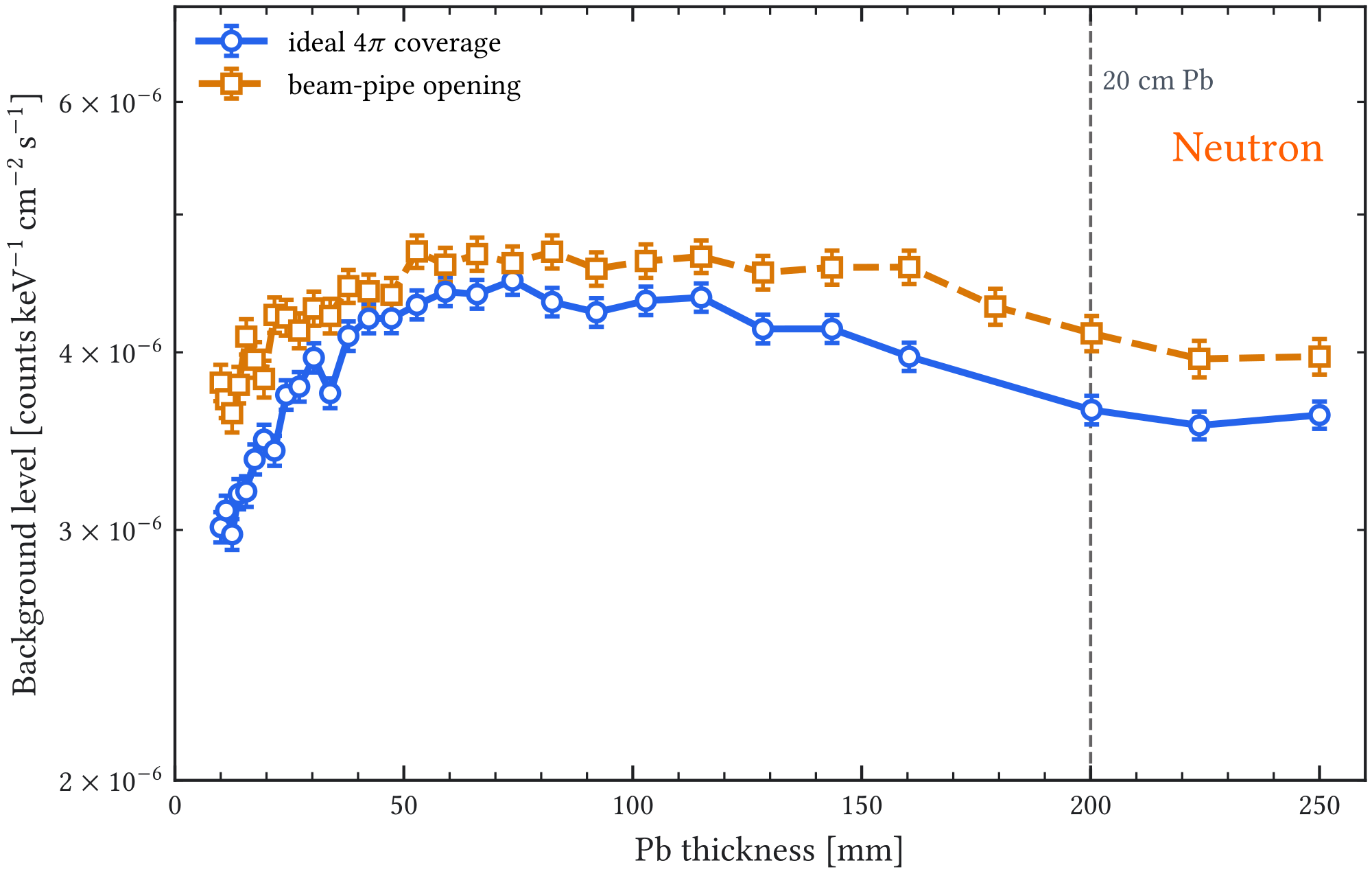
B Background-Model Source and Campaign Diagnostics
The source and campaign diagnostics preserve historical event counts and response mechanisms. Rate columns retain their original activity or source assumptions and analysis definitions; they are conditional scenarios rather than a common absolute inventory. In particular, cosmic exposure, source-angle and energy-range conventions require the campaign-ledger checks described in Section 6; historical prompt-veto rejection is not assigned to delayed activity.
A.1 Supplementary environmental-radioactivity plots
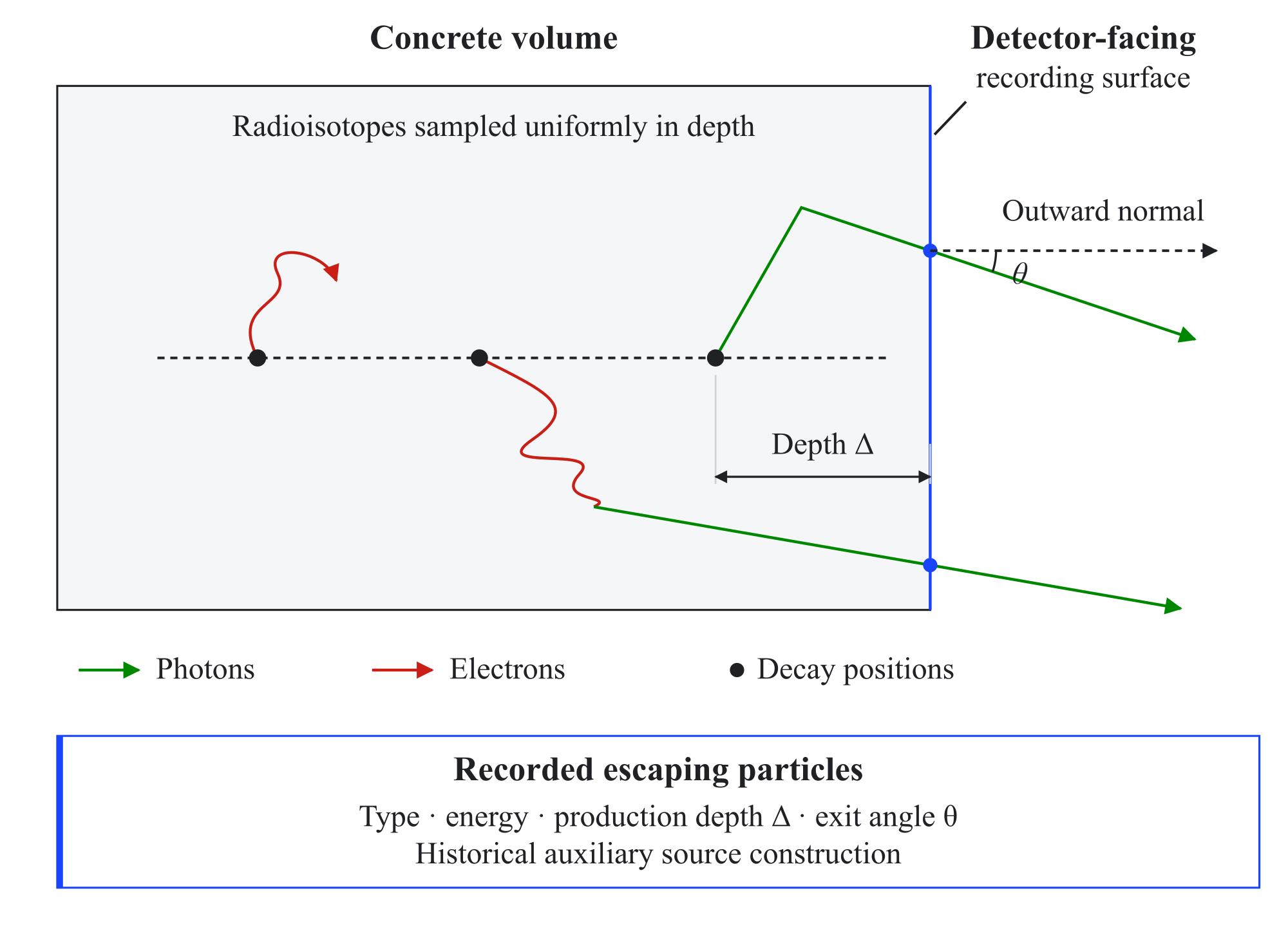
The background-model chapter now uses the concrete-radioactivity simulations mainly as provenance for the external-source methodology. The detailed plots are collected here because they document the earlier enclosed-laboratory source construction, even though they are no longer used as the nominal BabyIAXO site model.
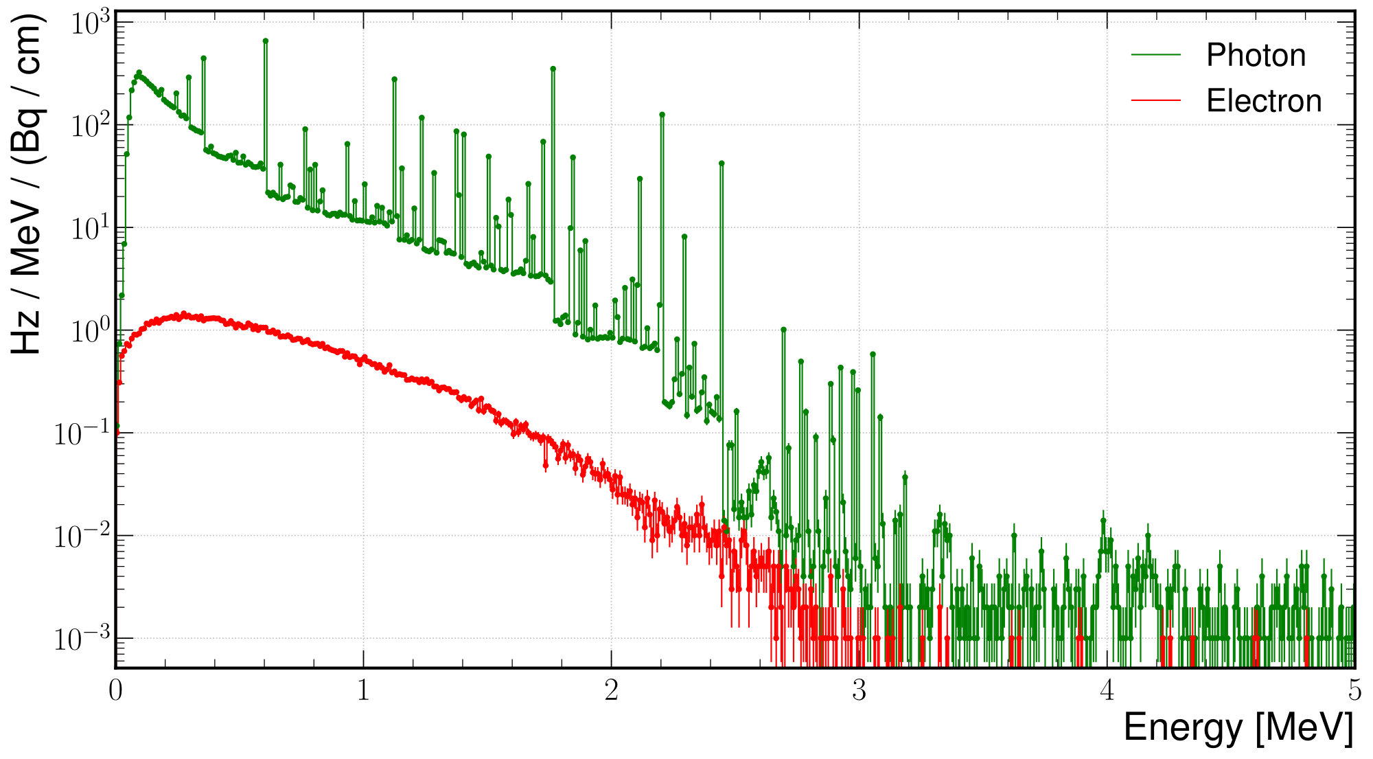
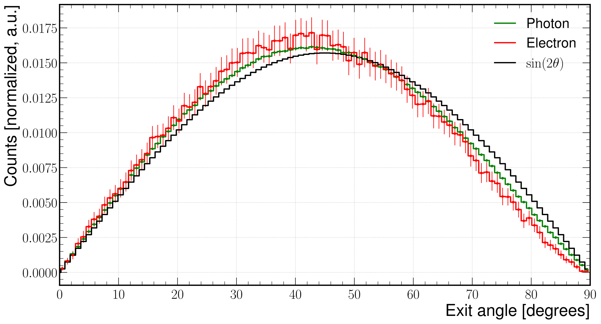
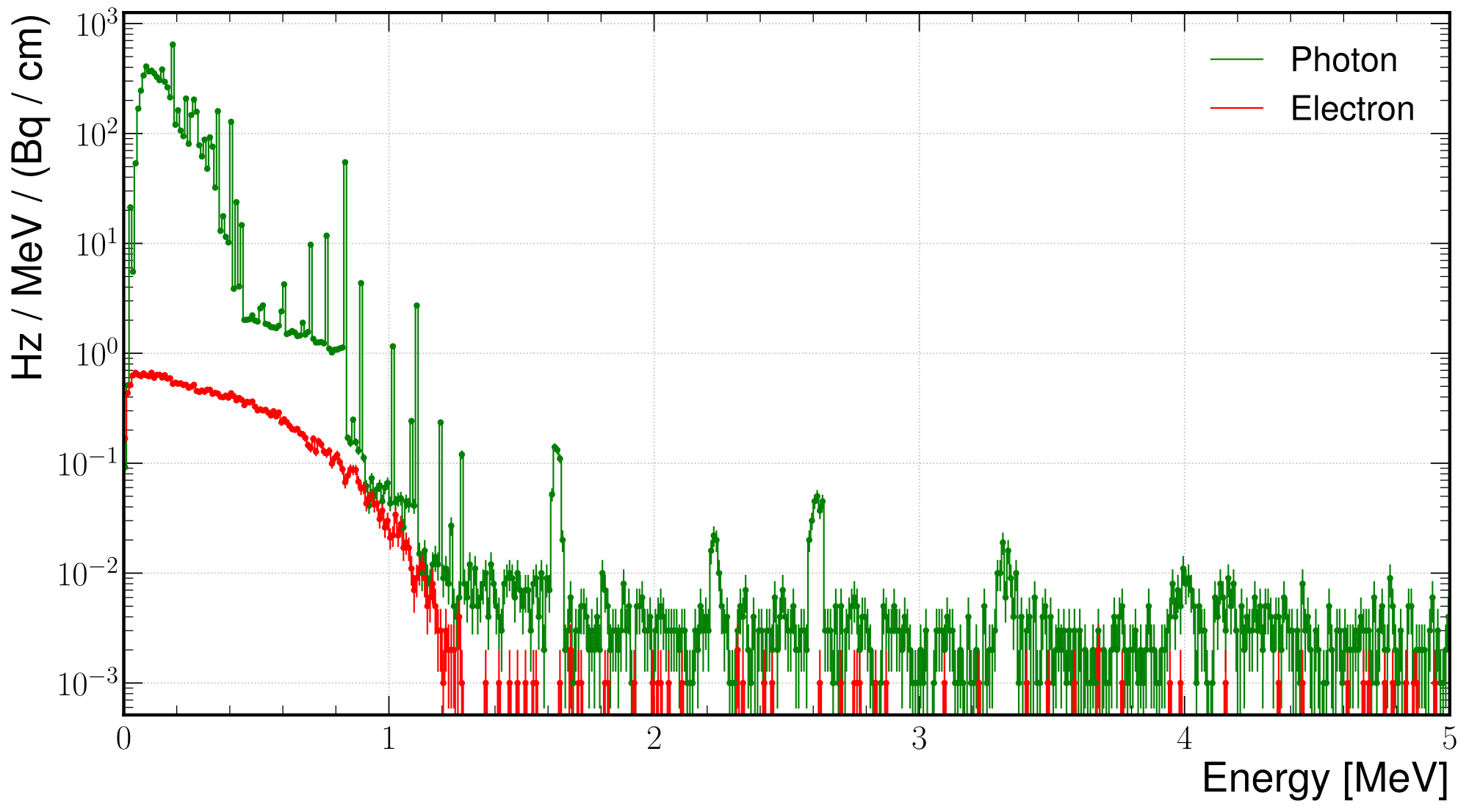
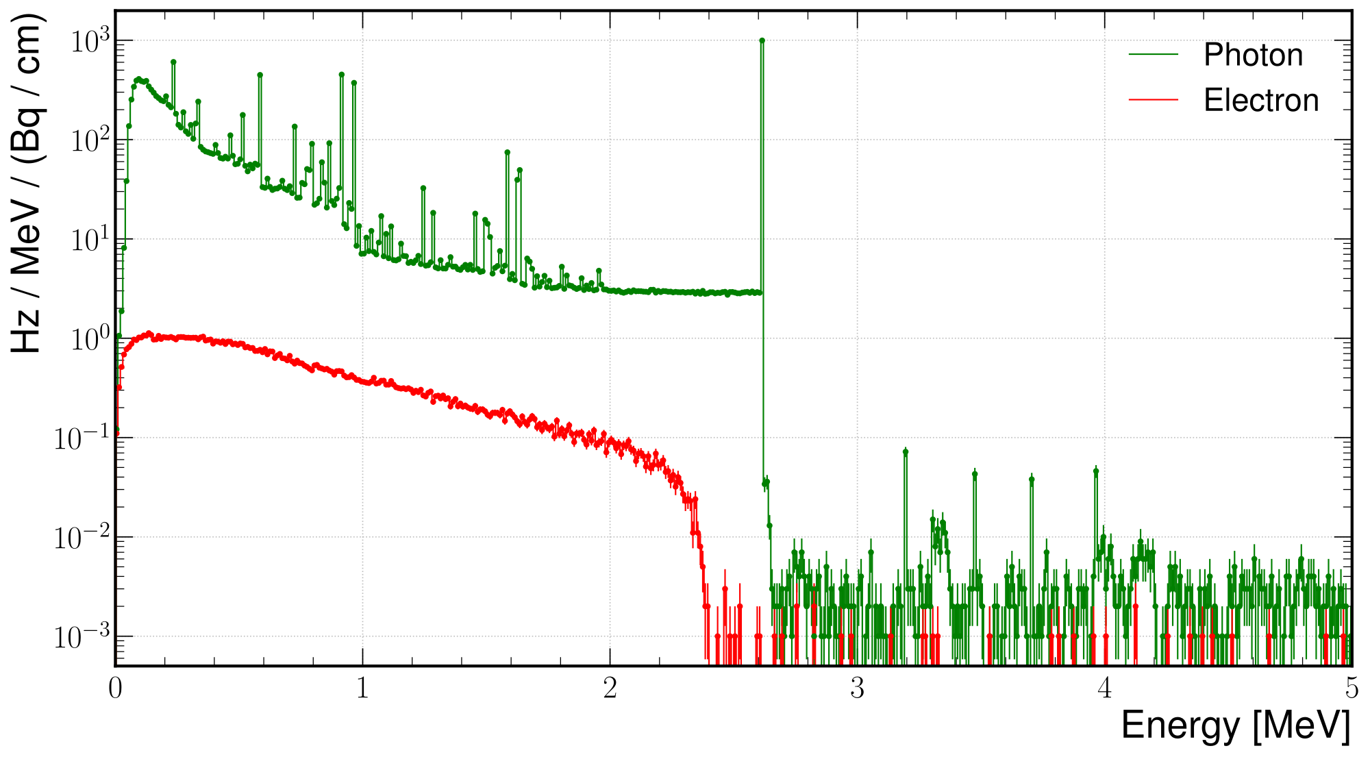
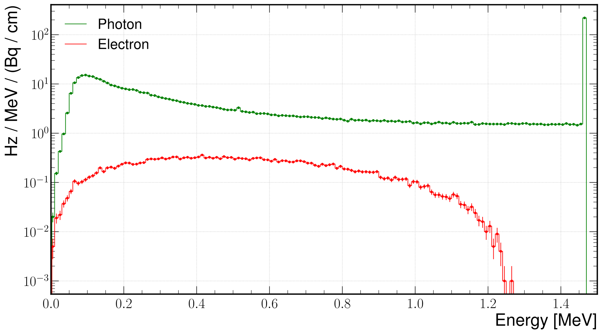
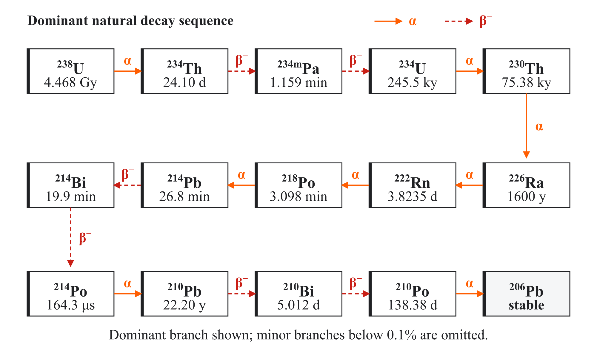
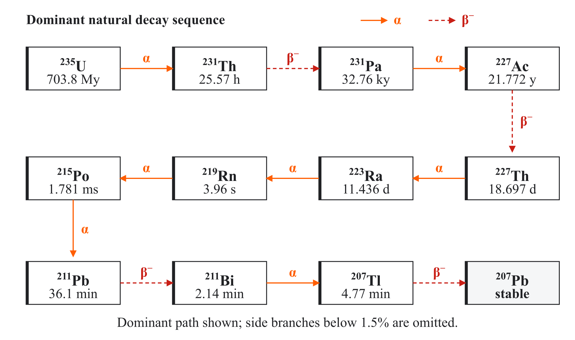
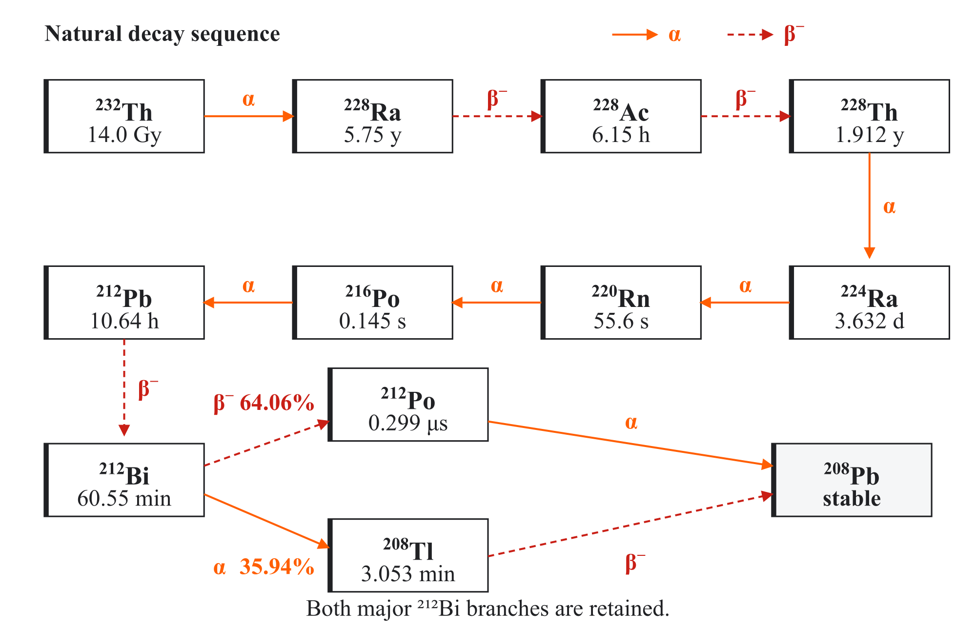
A.2 Environmental-radiation diagnostics
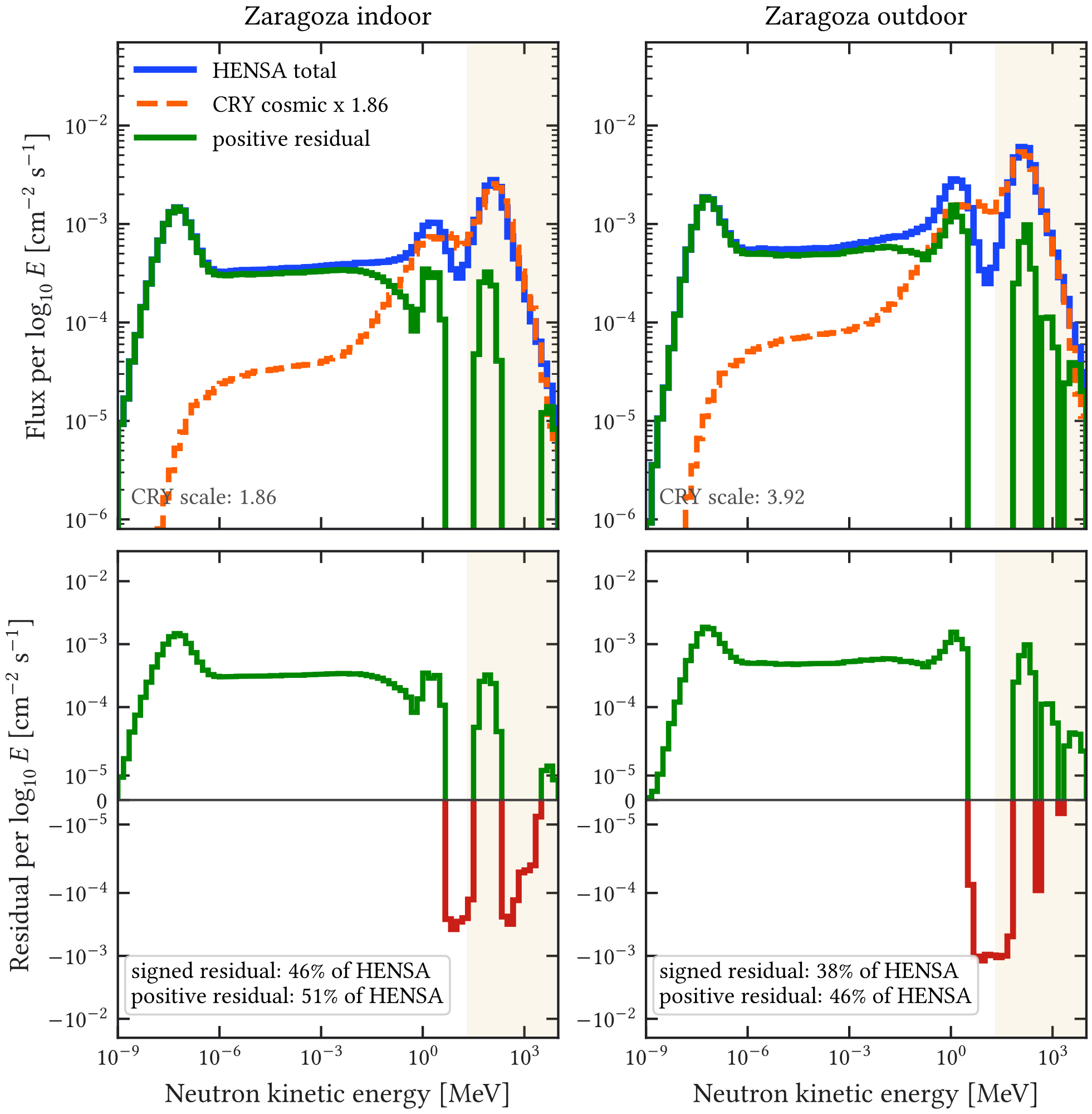
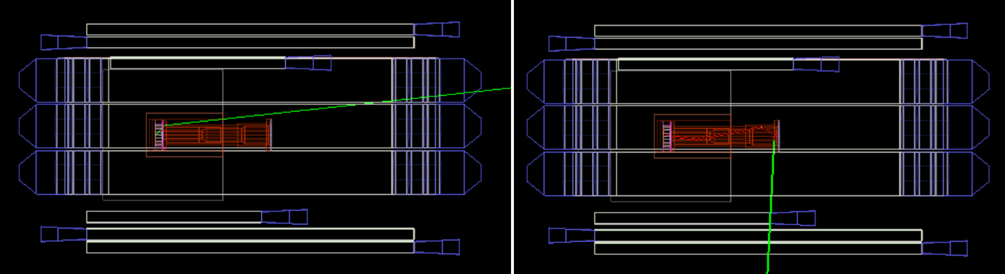
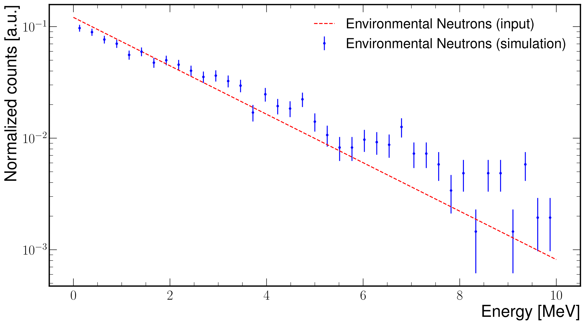
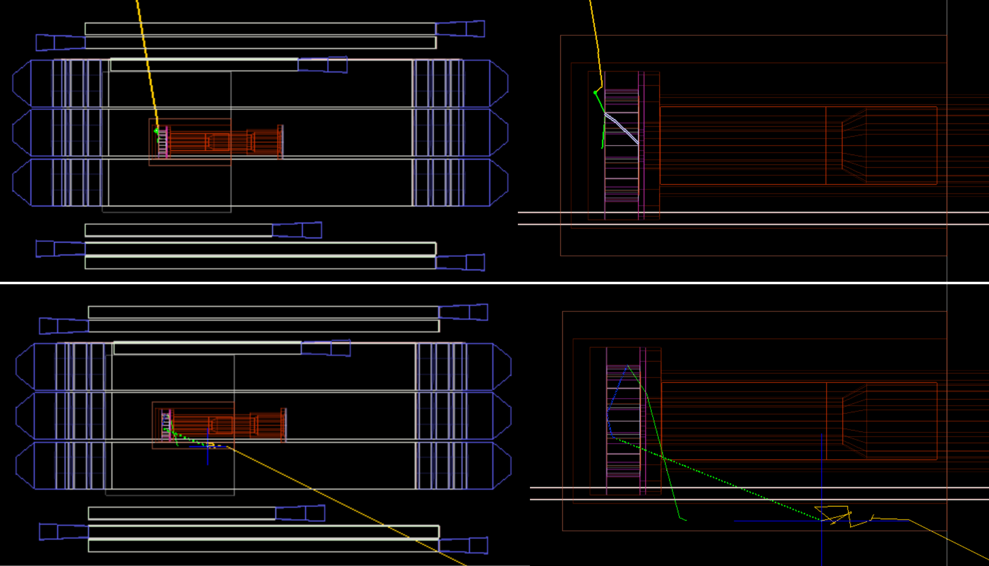
The plots below document the older environmental-gamma and environmental-neutron detector diagnostics. They are retained to show the interaction mechanisms and the evolution of the source model, but the current quantitative comparison in the background-model chapter uses the NaI-normalized gamma production and the HENSA-minus-CRY residual-neutron source.
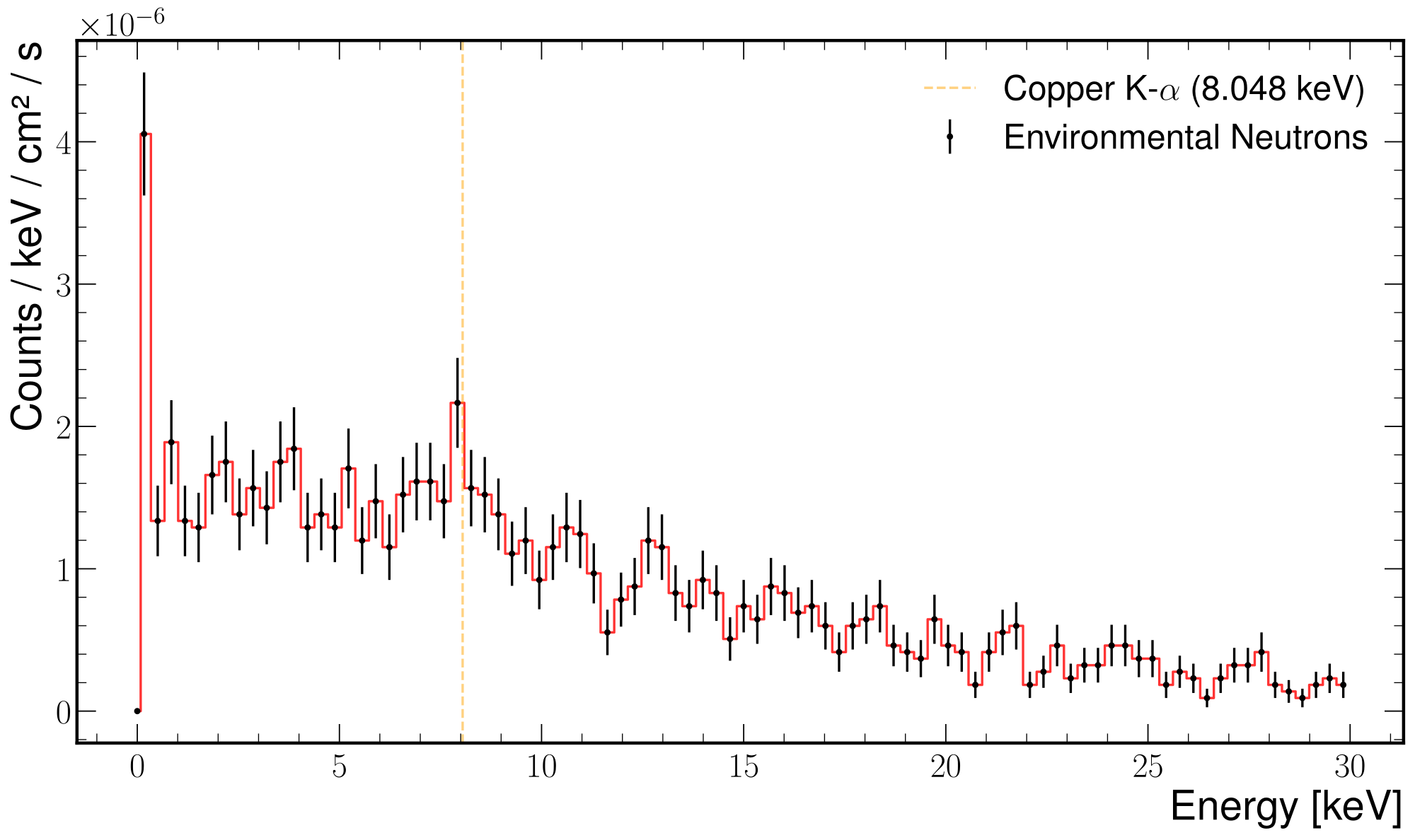
![Figure A.11: Reference energy spectrum of neutrons from spontaneous fission of 238 U [ 125 ]. This spectrum is retained as source-model context for radiogenic fast neutrons, but it is not used directly as the detector-level environmental-neutron input in the present background estimate. The main text instead uses the HENSA-minus-CRY residual environmental-neutron spectrum.](assets/bec019a18cb5e4e89909655b.png)
A.3 Supplementary intrinsic-shielding diagnostics
The shielding subsection in the background-model chapter quotes only the detector-level selection result. Table A.1 records the production snapshot behind that result in the same bookkeeping format used for the cosmic simulations. The equivalent physical time is computed from the generated decays and the adopted innermost-lead activity, .
| Source | Files | Disk [GiB] | CPU h | Decays | Eq. time [h] | Saved TPC | 2–7 keV |
|---|---|---|---|---|---|---|---|
| inner lead, 8 threads | 994 | 0.88 | 63616 | 6096 | 5937 | 1819 | |
| inner lead, 1 thread | 297 | 0.11 | 2376 | 205 | 210 | 64 | |
| inner lead, combined | 1291 | 0.99 | 65992 | 6301 | 6147 | 1883 | |
| inner lead, CuBox replaced by air | 100 | 0.13 | 6400 | 550 | 1455 | 429 |
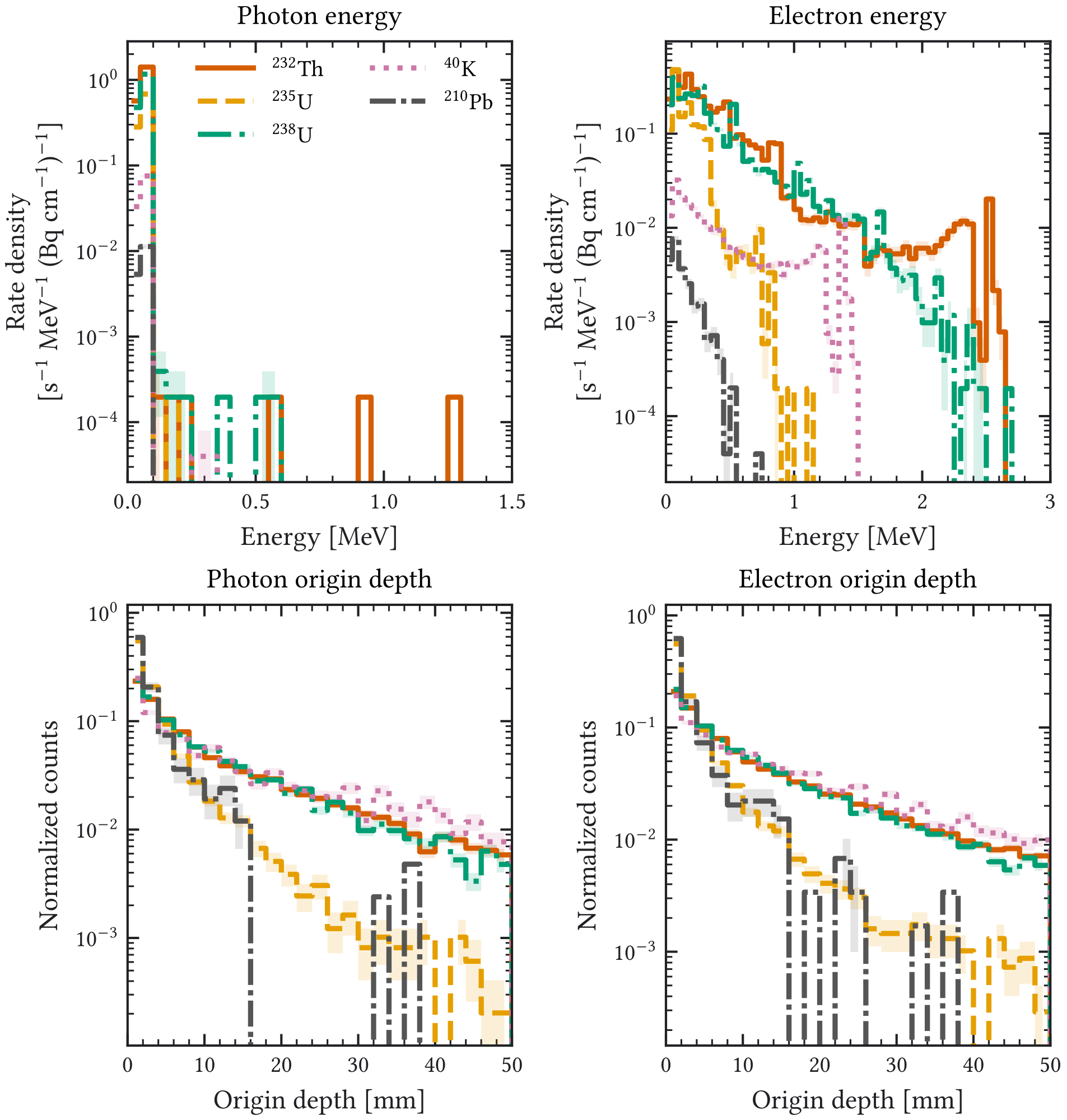
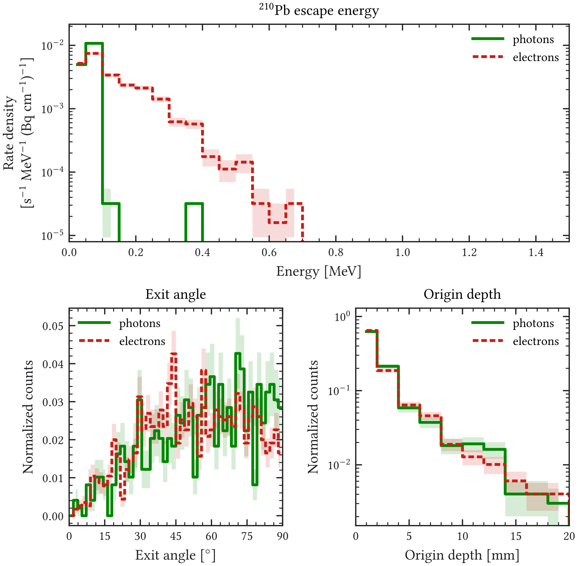
Geant4. “Saved TPC” gives the detector events written by the source filter, and the last column gives the fiducial – count after the common detector-response analysis. The CuBox-replaced-by-air row is a shielding-effect control sample and is not included in the combined nominal row.The following plots are retained as source-model diagnostics. They show why the detector-facing lead is the relevant source region for the electromagnetic shielding contribution, but the background level quoted in the main chapter is taken from the normalized detector-level production rather than from these transport-only distributions.
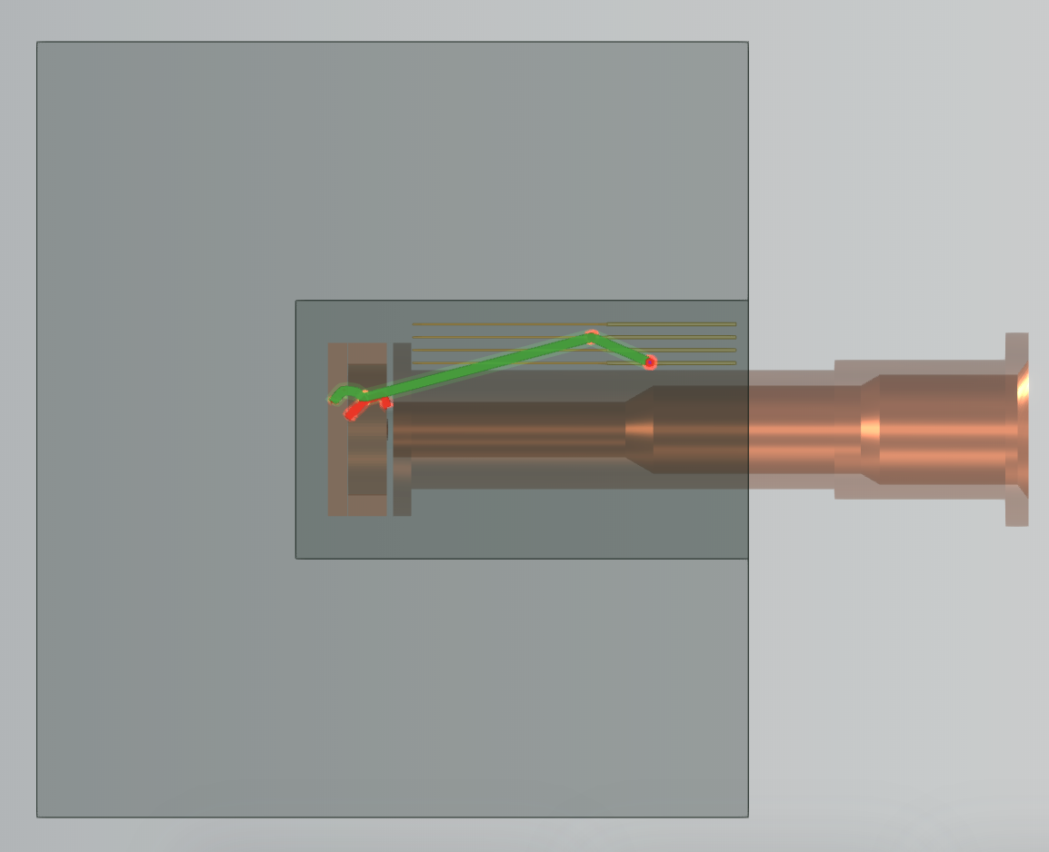
A.4 Supplementary electronics-card event diagnostic
A.5 Delayed-activation event-history diagnostics
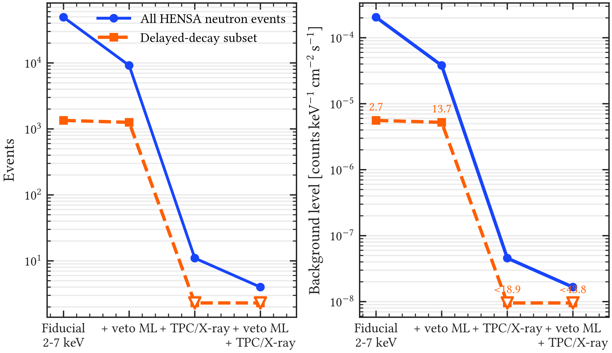
The delayed-decay label follows the event-history definition in Section 6.7. The diagnostic audit uses readoutEnergyInFiducial, a reconstructed-hit-centroid containment, and . It shares only the nominal – window and reporting units with the conservative partial inventory in Section 6; its response factors are not interchangeable with the maximum-track-center definition in Table 2.2.
| Cumulative selection | Delayed fraction | ||||
| 90% C.I. | 90% C.I. | 90% C.I. | |||
| Fiducial – | 49265 | 1346 | |||
| Fiducial – + veto ML | 9161 | 1258 | |||
| Fiducial – + full TPC/X-ray selection | 11 | 0 | |||
| Fiducial – + veto ML + full TPC/X-ray selection | 4 | 0 |
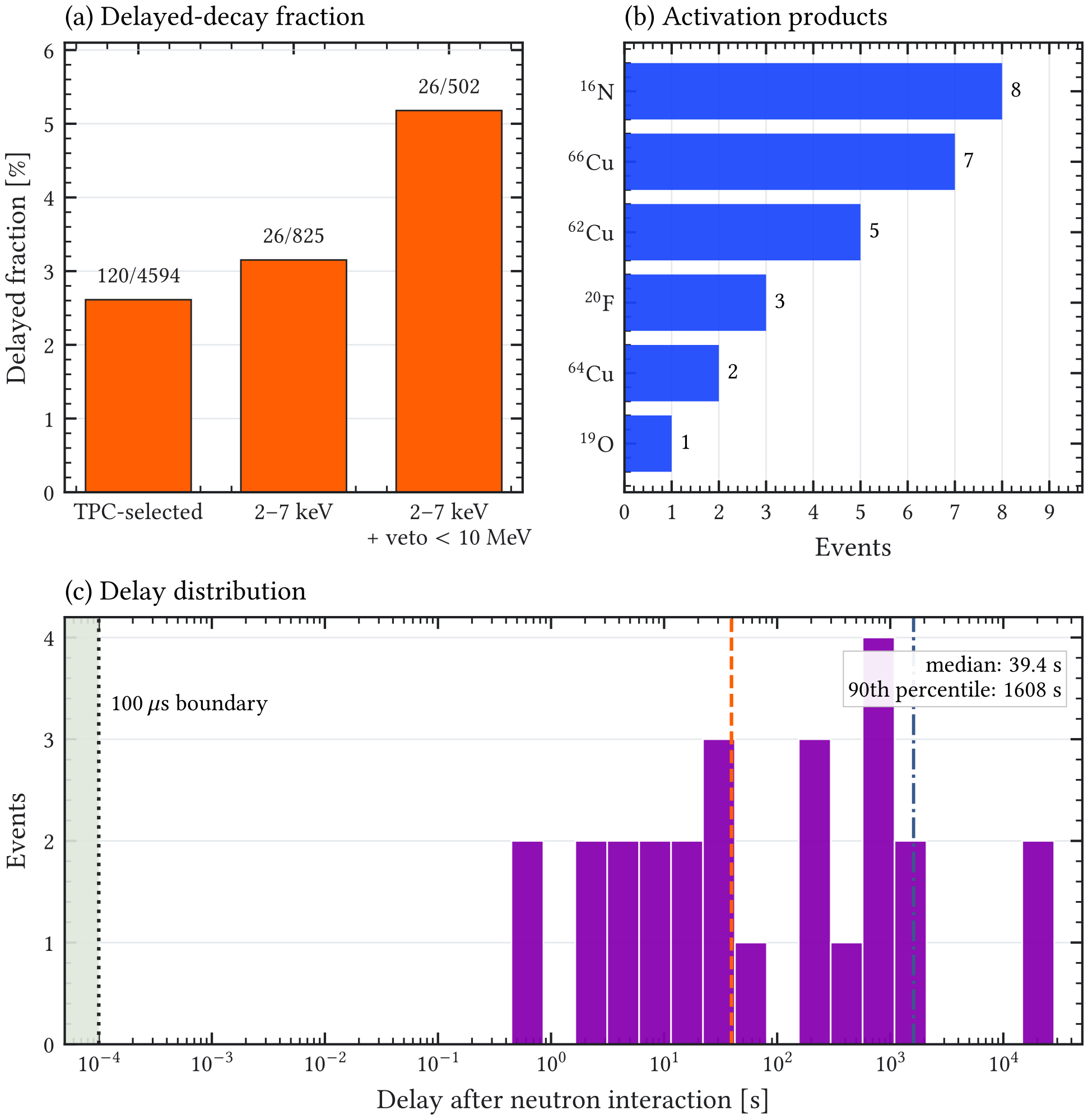
An independent earlier event-history diagnostic contains 4594 saved entries, of which 825 fall in the – region and 26 are classified as delayed decays. All 26 delayed events had no veto peak at the later Micromegas trigger and less than of reconstructed veto energy in that trigger window. The median delay was , or about , and the 90% quantile was , or about . The main activation products were (), (), (), (), (), and (). The half-lives are taken from the Geant4 radioactive-decay data used by the transport. The product count refers to the radioactive parent responsible for the delayed chain; subsequent daughter nuclei are not counted as additional activation products.
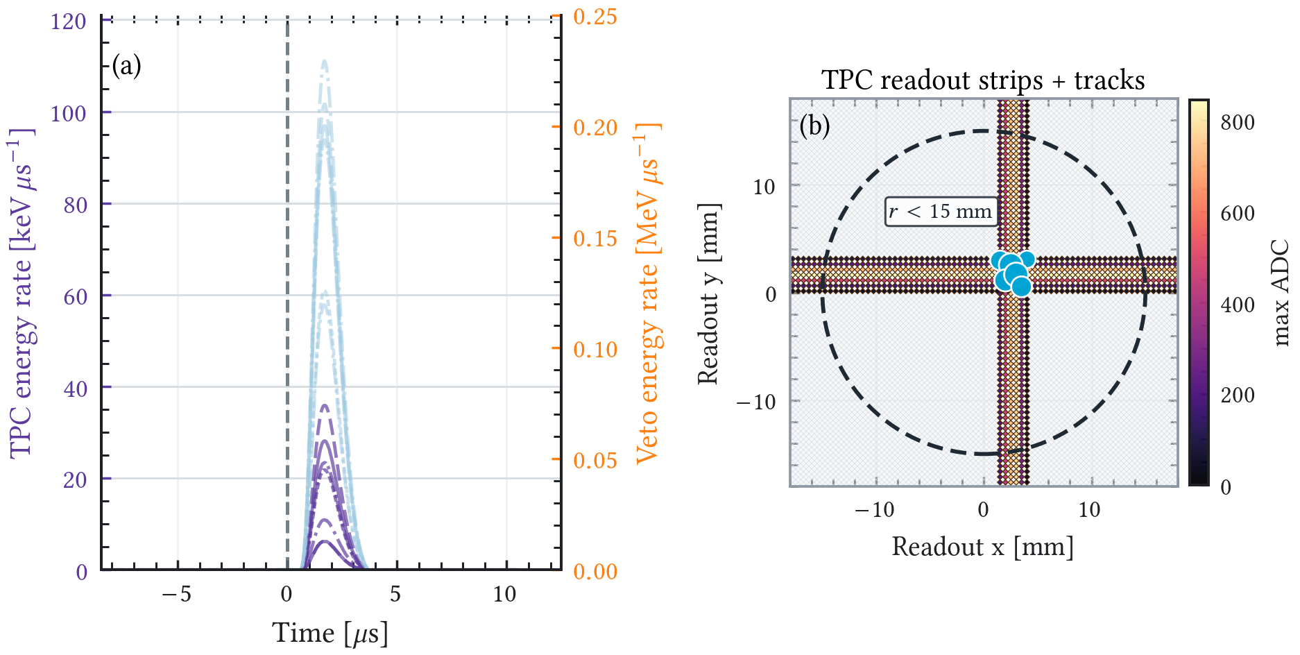
Before the reconstructed-hit fiducial requirement, one representative event passes the legacy fiducial-energy, veto, and X-ray BDT selections. The primary neutron produces a copper activation product; after , or , the decay chain emits a gamma that Compton-scatters an electron depositing energy in the gas. This event comes from the photon-evaporation audit sample, so its parent should not be read as one of the dominant products in Figure A.20; is the excited decay daughter.
| Quantity | Representative delayed survivor |
|---|---|
| Event identifier | output_494.root, entry , Geant4 event |
| Sample context | Photon-evaporation HENSA-neutron delayed-activation audit |
| Primary neutron energy | |
| Fiducial readout energy | |
| Total gas energy in the saved event | |
| Particle causing the TPC signal | Compton electron created by the delayed gamma; of gas energy |
| Activation parent and decay daughter | parent; excited daughter at |
| Reconstructed veto peaks at trigger | 0 |
| Reconstructed veto energy at trigger | |
| Delay after primary neutron interaction | |
| Causal chain | in gas |
The higher-statistics legacy survivor set contains 16 events, none with a delayed radioactive-decay ancestor in the survivor-level audit. Figure A.21 shows one after the legacy fiducial –, veto ML, X-ray BDT, and reconstructed-hit fiducial selections. Its gas energy is dominated by an elastic argon recoil, and the processed veto response is zero at the Micromegas trigger. It therefore represents the prompt no-veto tail rather than delayed activation.
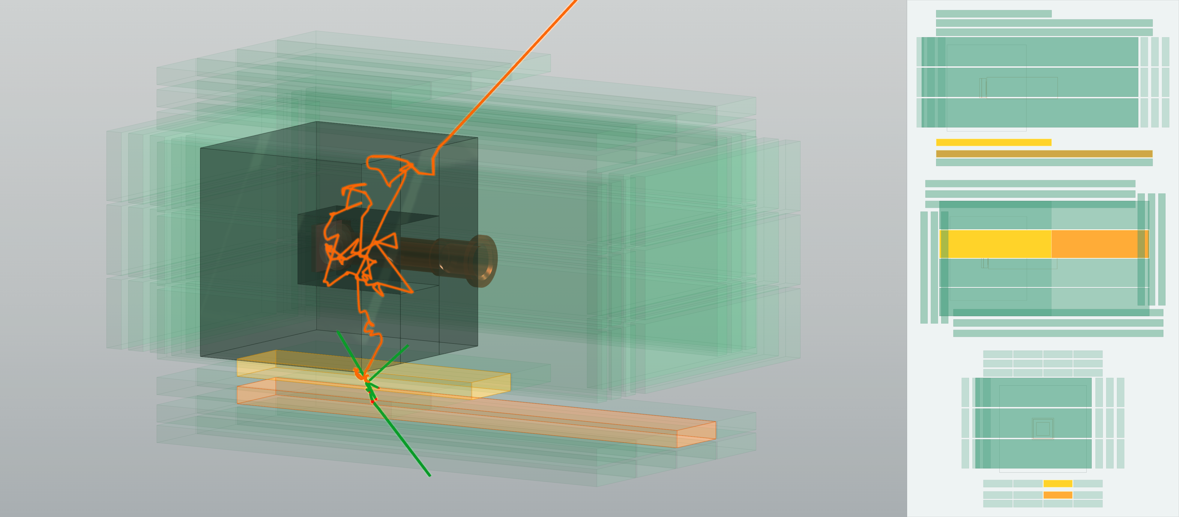
Geant4 event display with veto projections.A.6 Historical response-scale synthesis
The table below summarizes the physical interpretation and provenance of earlier source studies. It is supplementary because the rows use different historical selectors, source assumptions, and normalization areas. The entries are therefore not summed, and they are not a substitute for the deterministic partial inventory in Section 6.
| Source group | Retained evidence | Scope of inference |
|---|---|---|
| Gas and radon | Stored and selected counts; literature activity inputs in Table 2.9. | Earlier per-becquerel conversions are withdrawn because filtered stored entries were used as parent-decay denominators. |
| Electronics | Screened card activity vector and detector response under historical energy-binned cuts. | Cables, component placement, equilibrium assumptions, and deterministic-reference rescoring remain separate inputs. |
| Inner lead | Two survivors for the modeled shell and activity scenario. | Conditional historical bound; selected-event leakage from deeper lead has not been bounded. |
| Cosmic particles | Generated and selected event ledgers, including 249 HENSA candidates with three delayed histories. | Source yields are retained in Table 2.17; absolute source/exposure normalization is unresolved. |
| Activation | Production inventory and 73 selected dedicated cobalt decays. | Production-volume yields assume sampled spatial support; initial activity, irradiation, cooldown, and gas flow define a physical activity scenario. |
A.7 Background-model closure roadmap
Table A.5 records the analysis and source-model actions needed to extend the conservative IAXO-D1 partial inventory and, separately, to construct a BabyIAXO projection. Veto-specific optical response, channel mapping, thresholds, and online-logic uncertainties are owned by Section 5, especially Table 2.8, and are not repeated here.
| Uncertainty | Current treatment | Next action |
|---|---|---|
| Topology-model domain transfer | Candidate-v1 fails the measured gate; the bounded v2 family also fails non-blind background validation, selects no model, and leaves the blind block unopened. No learned topology rejection is credited. | Treat improved ML as optional future work requiring new independent run groups; deterministic detector-response validation remains necessary for the reference. |
| Signal efficiency versus energy | The complete ledger gives the reference-selection conservative response in 0.5-keV bins, peaking at for the specified calibration-like illumination. | For the separate BabyIAXO projection, repeat with Xe–Ne response, an optics-matched source, accidental-veto/live-time loss, and detector-response systematics. |
| Analysis harmonization and completeness | The registry records 30 physical sources: six generated-primary yields are available, while seven sources require reprocessing and sixteen require normalization, and seven require a source model or geometry. | Reprocess preserved outputs first; resolve detector-specific inputs next; simulate only genuinely missing sources; never treat omitted rows as zero. |
| Gas activity and radon plate-out | Literature activity scenarios for and are stated independently of response normalization; radon and progeny retain stored counts pending generated-parent denominators. | Recover parent-decay denominators and replace scenario activities with detector-specific gas assays, emanation measurements, and surface-history constraints when available. |
| Cosmic-neutron normalization | The outdoor HENSA 10 GeV spectrum supplies contract-compatible prompt/non-delayed and activation leaf responses; the latter has a conditional yield bound and an independent production-volume decay study. Absolute rates require source-area, angular, and energy-range closure. | Validate prompt-veto rejection only for the prompt channel, retain zero prompt-veto credit for activation, and transfer the source field to the selected site scenario. |
| Zaragoza/DESY site dependence | Zaragoza and DESY latitudes are considered in the cosmic-source setup, but not all final DESY boundary conditions are fixed. | Produce a DESY-specific source term once the site configuration is frozen. |
Geant4 hadronic modeling | High-precision neutron and binary-cascade models are used consistently across source classes. | Compare key neutron observables across relevant physics-list choices. |
| Finite Monte Carlo statistics | The reporting convention gives central 90% intervals above two counts and one-sided bounds at zero, one, or two. This mixed display is not one unified coverage construction. | Increase independent exposure only where a conservative-reference bound remains decision-relevant after the geometry and source term are fixed. |
A.8 Cosmic-simulation campaign metadata
The cosmic-background discussion in the background-model chapter uses compact source labels and cut-flow tables. Table A.6 records the production-level snapshot behind those results. The table is a bookkeeping table, not a background-level table: it lists completed ROOT files, generated primaries, and the number of detector events available to the fiducial – selection. The earlier equivalent-time column is omitted because the preserved cut-flow calculation used hardcoded rates, while the campaign-matched source-area and energy-acceptance ledger remains incomplete. In particular, the former neutron entry of 1031 hours was not the time in its source CSV: that value was approximately the numerical generation rate in inverse seconds. The counts below remain independent of that conversion. The CRY light-particle rows and the Guan muon row correspond to the current -shape all-cosmic snapshot. The HENSA aggregate row supplies the current pre-veto yield and its matched 249-event prompt/delayed partition in Table 2.17. The independent higher-statistics history audit remains a separate legacy diagnostic.
| Primary | Snapshot | Files | Primaries | TPC selected | Snapshot fiducial | Snapshot final |
|---|---|---|---|---|---|---|
| -shape | 454 | 1031 | 1 | 0 | ||
| -shape | 499 | 231 | 1 | 0 | ||
| -shape | 221 | 14586 | 44 | 0 | ||
| Guan muons | -shape | 1495 | 1742989 | 0 | 0 | |
| HENSA | conservative aggregate | 1750 | 108833 | 249 | — | |
| history audit | 4585 | 403284 | 124328 | 16 |
Geant4. “TPC selected” gives the detector events written by the restG4 source filter and retained by the corresponding flat-feature analysis. The final columns are snapshot specific. For the light-particle and Guan rows, the fiducial column is the conservative maximum-track stage, whereas the final column is retained only as a candidate-v1 topology/veto diagnostic. The aggregate HENSA row supplies the conservative pre-veto response and therefore has no credited final-selection entry. The history-audit row instead uses the legacy hit-centroid, topology, and veto definition required for the prompt/delayed split.A.9 Supplementary cosmic-source mechanisms and detector-response diagnostics
The background-model chapter retains the physical source routes, deterministic fiducial responses, and source-level conclusions. This section records the truth-history classification, historical topology and veto cut flows, representative event displays, and the muon fiducial-position diagnostic. These results support mechanism interpretation and analysis provenance, but they do not supply topology or veto-rejection credit to the conservative reference.
All rate columns in this appendix retain the historical source/exposure conversion for reproducibility. They are conditional normalization scenarios rather than validated absolute bounds: the muon generation area, HENSA energy-range acceptance and angular encoding, and matched campaign inventory must first be recovered. Event counts and truth-history classifications remain usable independently of that conversion. The labels of the original tables are shortened to “Guan muons” because the local source configuration emits only negative muons and the archived charge composition has not been established.
A.9.1 CRY truth-history classification
To identify the physical origin of Micromegas deposits, a separate event-history classification was applied to higher-statistics processed CRY gamma, electron/positron, and proton diagnostic samples. For each event, the track depositing the largest energy in the Micromegas signal volume, Chamber_gasAboveReadout, was identified and its parent track IDs were followed back to the primary particle. The resulting categories are summarized in Table A.7. This classification uses the Geant4 truth history only to interpret the mechanism; the detector-response cut flows remain based on reconstructed observables.
| Source | Dominant TPC-depositing track | Events | Event fraction | TPC-energy fraction | Interpretation |
|---|---|---|---|---|---|
| CRY gammas | Secondary | 7882 | Photon converts or Compton-scatters, directly or after an electromagnetic shower; the charged lepton ionizes the gas. | ||
| CRY gammas | Other secondary | 97 | Rare photonuclear chains create neutron, proton, or nuclear-recoil descendants that reach the gas. | ||
| CRY e | Electromagnetic shower secondary | 30 | The primary radiates bremsstrahlung photons, which convert or Compton-scatter into the charged particle that deposits in the gas. | ||
| CRY e | Primary | 1 | Direct ionization by the generated charged lepton. | ||
| CRY protons | Electromagnetic secondary | 2684 | Proton-induced cascades produce photons and electrons; the gas signal is usually deposited by an . | ||
| CRY protons | Secondary proton or elastic recoil | 1656 | Hadronic interactions in the shielding or chamber create lower-energy protons that ionize the gas efficiently. | ||
| CRY protons | Primary proton | 983 | The generated proton itself reaches the Micromegas gas and deposits energy by ionization. | ||
| CRY protons | Charged cascade particle | 590 | Charged pions, muons, or related cascade products cross the gas after a hadronic interaction. | ||
| CRY protons | Neutron or nuclear-fragment descendant | 257 | Secondary neutrons and light nuclear fragments are uncommon, but some recoil fragments carry large local ionization. |
CRY gamma, electron/positron, and proton diagnostic samples. The event fraction is computed within each source class after requiring a non-zero Micromegas signal. The TPC-energy fraction is the fraction of the total energy deposited in the Micromegas signal volume by the dominant track category. This table is used for mechanism interpretation; the normalized final-selection rates are taken from the current -shape detector-response snapshot in Table A.8.The gamma result is the cleanest: the primary photon is almost never the particle that deposits the signal energy. It first produces an electron or positron through Compton scattering, pair conversion, or a short electromagnetic shower; the charged secondary then creates the gas ionization. The electron/positron source behaves similarly, except that the shower starts from a charged primary and often proceeds through bremsstrahlung photons before returning to an electron-like gas deposit. The proton source is more mixed. By event count, electromagnetic descendants are the largest class, but hadronic or elastic proton secondaries and nuclear fragments account for a larger fraction of the deposited TPC energy.
A.9.2 CRY detector-response and event-display diagnostics
| Source | Cumulative selection | Events | Background level with 90% C.I. |
|---|---|---|---|
| CRY gammas | TPC selected | 1031 | |
| CRY gammas | Full readout 2–7 keV | 328 | |
| CRY gammas | Fiducial 2–7 keV | 1 | |
| CRY gammas | Fiducial 2–7 keV + veto ML + interval topology | 0 | |
| CRY gammas | Fiducial 2–7 keV + veto ML + BDT topology | 0 | |
| CRY e | TPC selected | 231 | |
| CRY e | Full readout 2–7 keV | 77 | |
| CRY e | Fiducial 2–7 keV | 1 | |
| CRY e | Fiducial 2–7 keV + veto ML + interval topology | 0 | |
| CRY e | Fiducial 2–7 keV + veto ML + BDT topology | 0 | |
| CRY protons | TPC selected | 14586 | |
| CRY protons | Full readout 2–7 keV | 3871 | |
| CRY protons | Fiducial 2–7 keV | 44 | |
| CRY protons | Fiducial 2–7 keV + veto ML + interval topology | 0 | |
| CRY protons | Fiducial 2–7 keV + veto ML + BDT topology | 0 |
CRY gamma, electron/positron, and proton productions in the current -shape analysis snapshot. Background levels are in . The first two rate rows are normalized to the full readout area; rows beginning with the fiducial selection are normalized to the -radius axion-window area. Ordinary-count rows give central levels with two-sided 90% Garwood intervals; rows with zero, one, or two survivors give one-sided 90% confidence upper bounds. The veto-bearing rows score source frames without the calibration-noise overlay used to define the diagnostic veto classifier and are therefore domain-mismatched. The topology rows also use a simulation-trained selector that fails its measured-signal efficiency gate. Both are excluded from the conservative partial reference.In the domain-mismatched diagnostic columns, no gamma, electron/positron, or proton event survives the combined veto and X-ray-topology selections in the current normalized productions. Of the 44 proton-induced events entering the fiducial energy window, one remains after the diagnostic veto classifier before the topology cut. This pattern is qualitatively compatible with prompt scintillator activity from the charged primary, but it is not a validated proton-veto efficiency. The electron/positron and gamma samples each contain one fiducial event and zero final topology survivors. These observations motivate future source-specific topology studies, but they do not provide a credited rejection factor in the conservative reference.
| Source | Selected example | Veto peaks | Selection outcome | ||
|---|---|---|---|---|---|
| CRY gamma | Compact Micromegas deposit inside the fiducial circle | 0 | Veto passes; full TPC/X-ray rejects | ||
| CRY e | Fiducial-energy event with a charged-particle veto response | 3 | Veto rejects; full TPC/X-ray rejects | ||
| CRY proton | Fiducial-energy event with large prompt veto activity and reconstructed hits outside the circle | 324 | Veto rejects; full TPC/X-ray rejects |
CRY gamma, electron/positron, and proton benchmark events selected for visual inspection. These visual examples were selected with the earlier hitsReadoutAnalysisAfter_readoutEnergyInFiducial and diagnostic definition; they illustrate event mechanisms and do not define the conservative thesis reference. The veto energy is the reconstructed rawPeaksVETO energy sum after detector-response processing.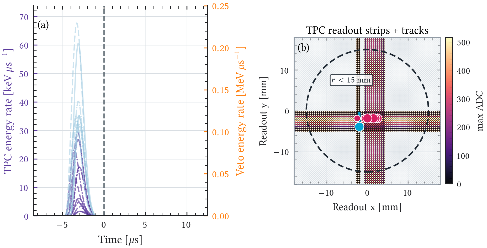
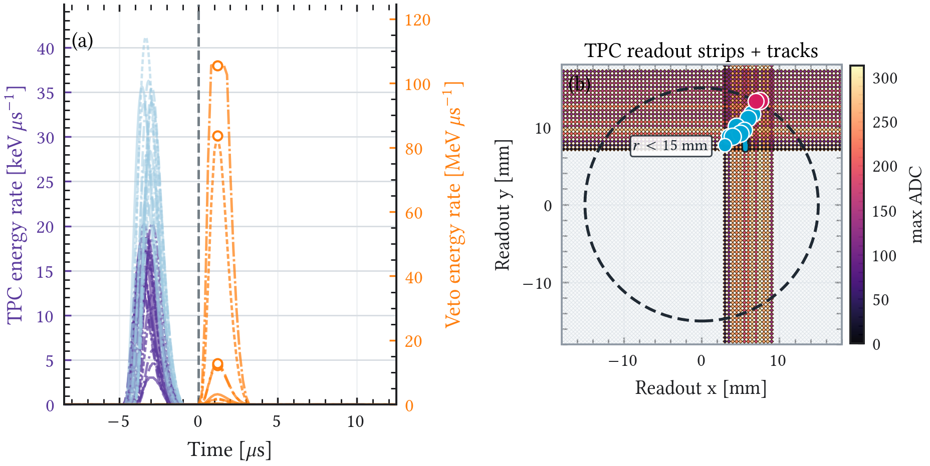
CRY gamma and electron/positron benchmark events after detector-response processing. Each panel shows the Micromegas and veto waveforms on the left and the active readout strips with reconstructed tracks on the right. Together with Figure A.23, these examples illustrate why the components are retained in the cosmic-ray catalog even though the current normalized productions have no full-selection survivor.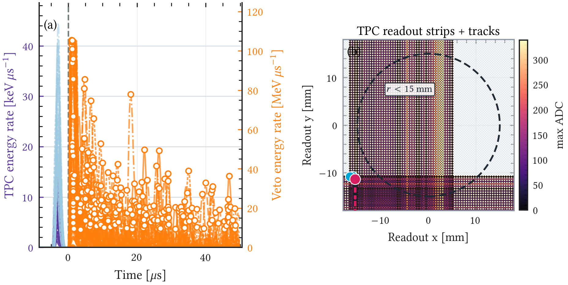
CRY proton benchmark event after detector-response processing. The Micromegas and veto waveforms are shown on the left and the active readout strips with reconstructed tracks on the right.A.9.3 Historical common cut flow and muon fiducial diagnostic
Table A.10 retains the topology and veto branches of the background-analysis-v1 diagnostic. The samples were processed with the -tuned detector-response snapshot and the same reconstruction chain used for the conservative inventory. The BDT columns use grouped out-of-fold scores for development campaigns and the development-only frozen deployment model for production-holdout campaigns. The first two stages retain the full readout; the fiducial and later stages require a reconstructed track center within of its center.
| Source | Energy | +track | Fid. | ||||
| BDT | |||||||
| +interval | |||||||
| +group-safe | |||||||
| BDT | |||||||
| CRY | 77 | 21 | 1 | 0 | 0 | 0 | 0 |
| CRY | 328 | 84 | 1 | 0 | 1 | 0 | 0 |
| Guan muons | 1484 | 1014 | 0 | 0 | 0 | 0 | 0 |
| HENSA | 23382 | 13916 | 249 | 29 | 53 | 5 | 8 |
| CRY | 3871 | 2259 | 44 | 2 | 7 | 0 | 0 |
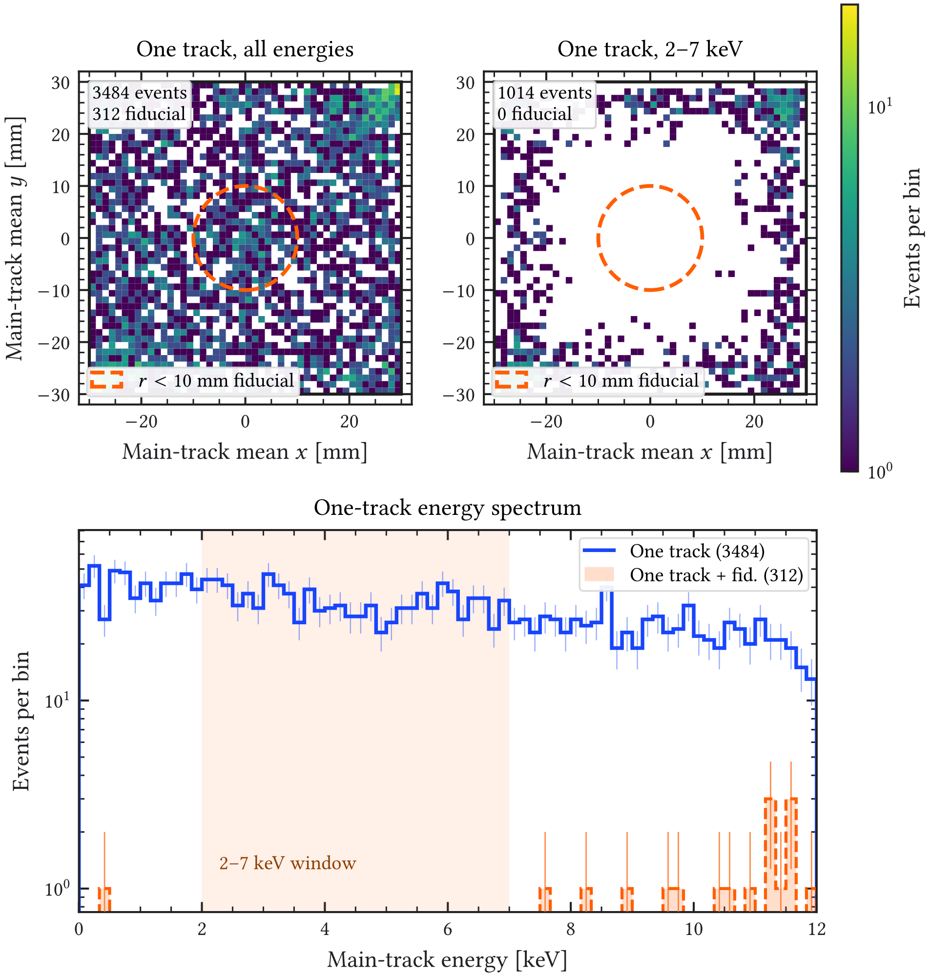
background-analysis-v1 cross-fit/holdout diagnostic. The first three stages apply reconstructed energy, one track per projection, and fiducial containment in sequence. The interval and group-safe BDT columns are alternative Micromegas-topology branches after the fiducial stage; the final two additionally apply the veto classifier. These veto columns omit the calibration-noise overlay used to construct that classifier and therefore remain domain mismatched. The fiducial counts and selection match Table 2.17, which supplies generated-primary yields and the matched 249-event HENSA prompt/delayed partition. The unverified historical conversion to absolute background levels is not retained. No topology rejection is credited in the reference selection: the simulation-trained selector retains only of the measured R02756 check. Table 2.23 records the separate, higher-statistics legacy history audit.Figure A.24 gives the corresponding diagnostic for the updated Guan-fix muon sample. The upper-left panel shows the reconstructed center of the dominant track for all events with one reconstructed track in each strip projection, before imposing the energy window. The lower panel gives the corresponding one-track energy spectrum and compares the full readout with the -radius fiducial subset. The upper-right panel shows the one-track position map after the – requirement; these events are concentrated near the readout edge and none lies inside the fiducial circle.
C Background-Model Analysis and Response Diagnostics
A.1 Reconstruction and X-ray-selection validation
The main background-model chapter retains the physical reconstruction chain, the decisive selector-validation results, and the decision not to credit topology rejection in the conservative reference. The material collected here records the event-container sequence, detector-response parameterization, exact reconstruction-process inventory, reference samples, classifier observables, run-block checks, and legacy candidate-v1 response needed for reproducibility. They do not define an additional rejection factor in the thesis background level.
A.1.1 Event-container and reconstruction gallery
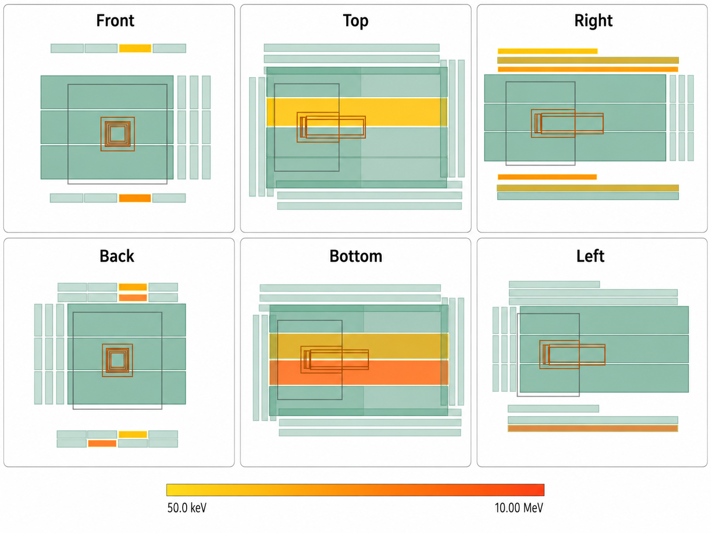
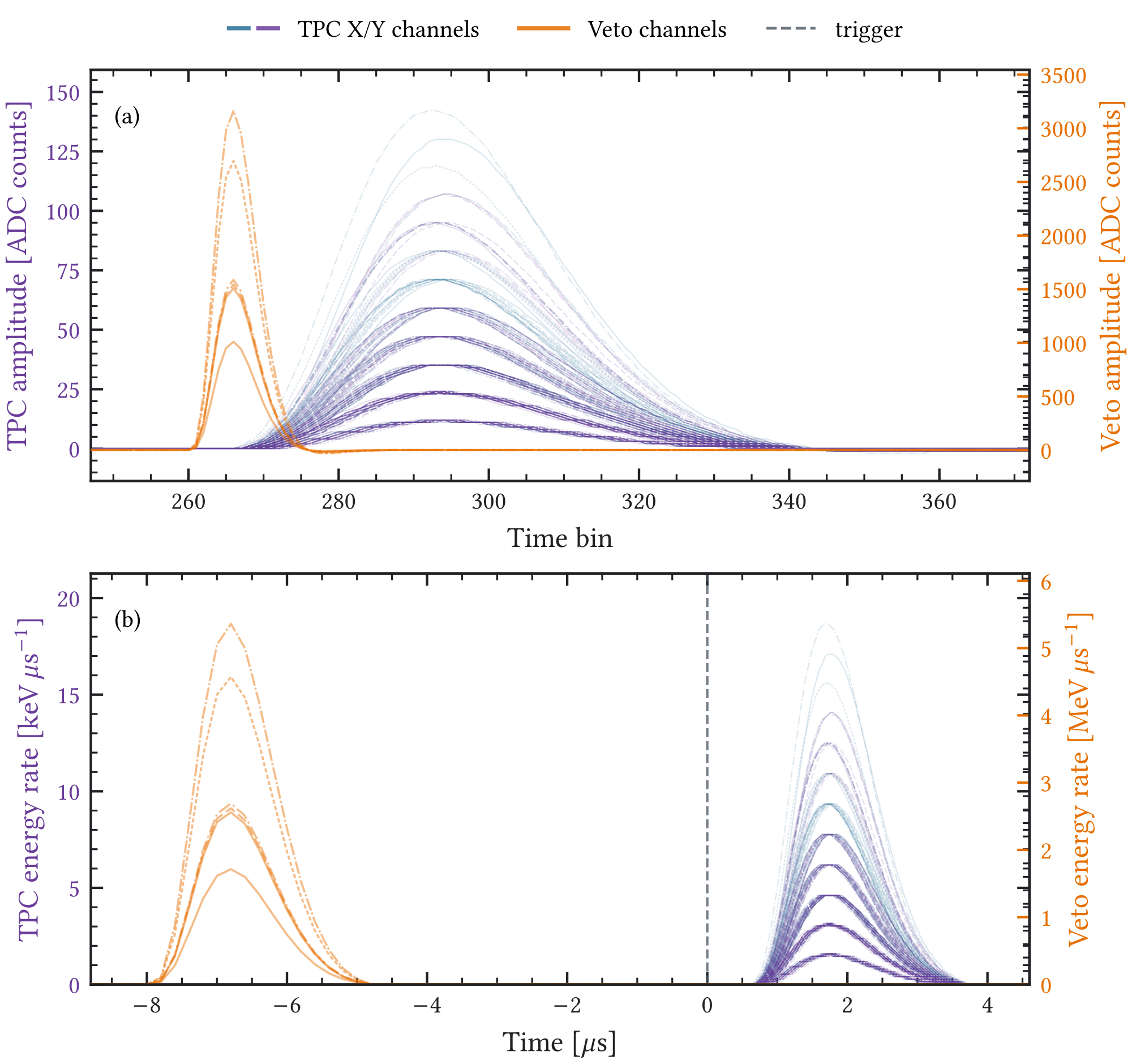
The main chapter summarizes the transition from Geant4 truth to reconstructed analysis observables. The displays below show intermediate event representations for several simulated cosmic-muon examples.
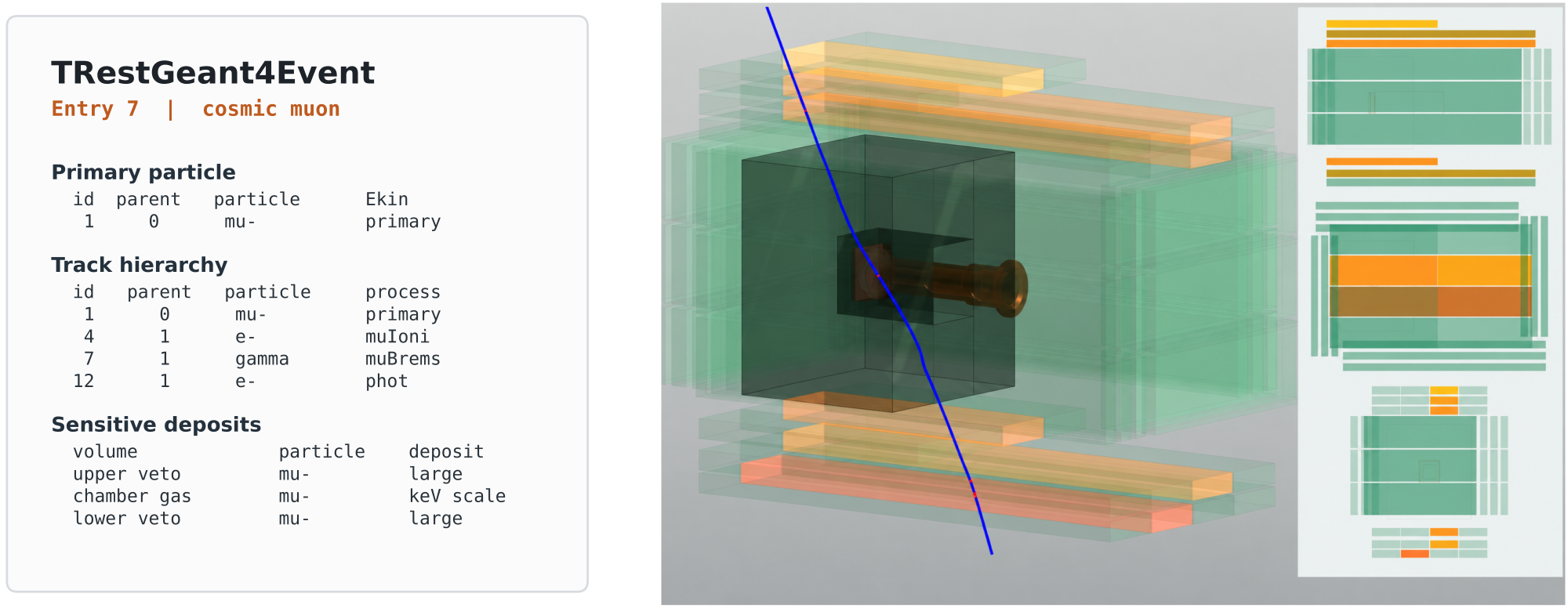
TRestGeant4Event summary, while the right panel shows the corresponding transport event in the detector and veto geometry before detector-response emulation.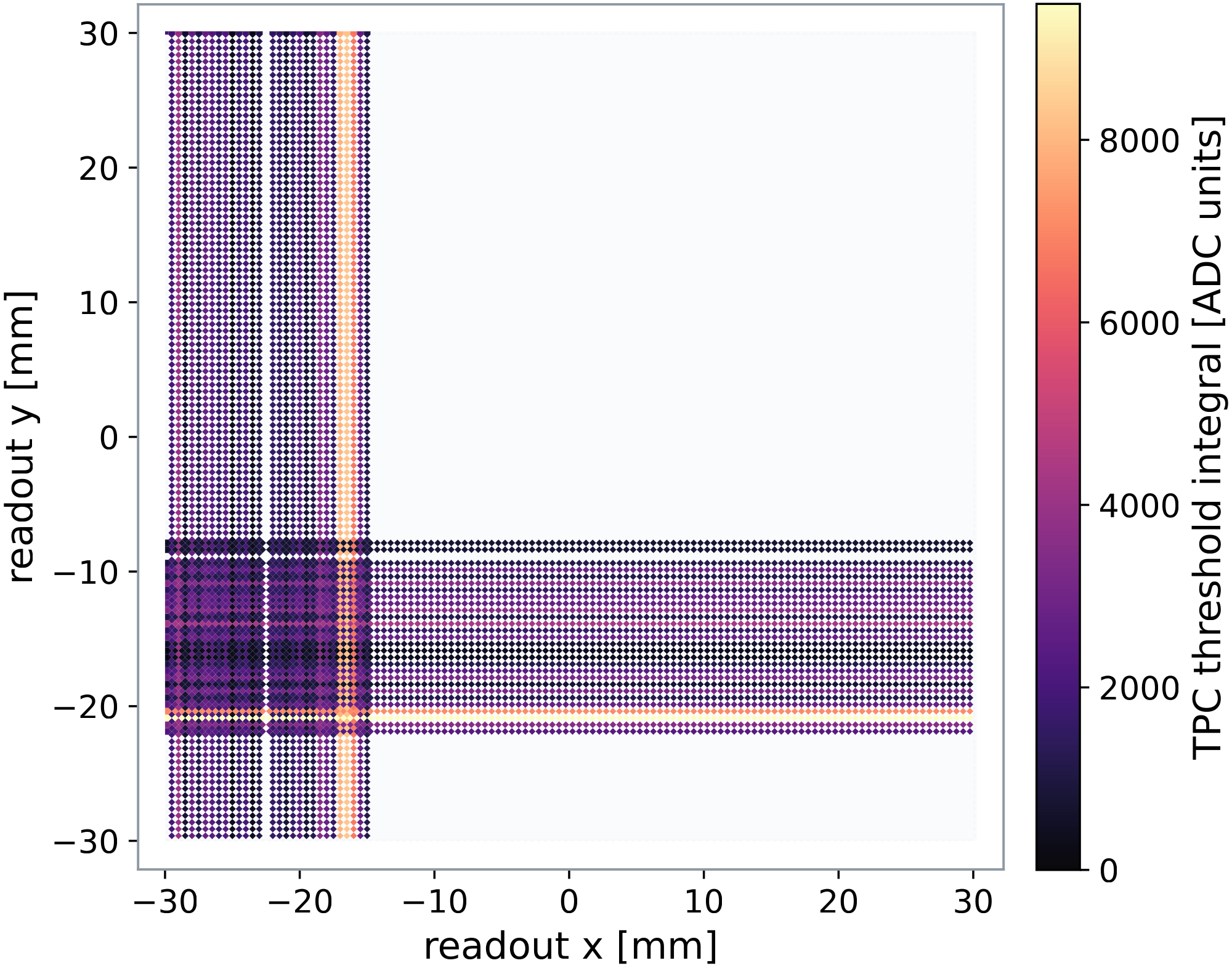
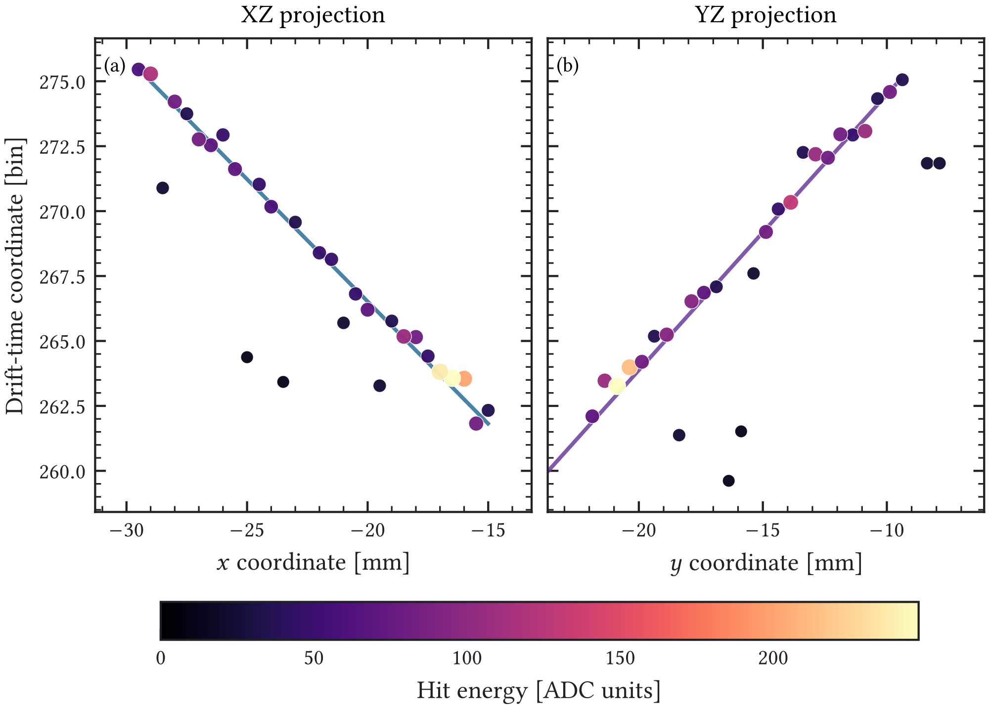
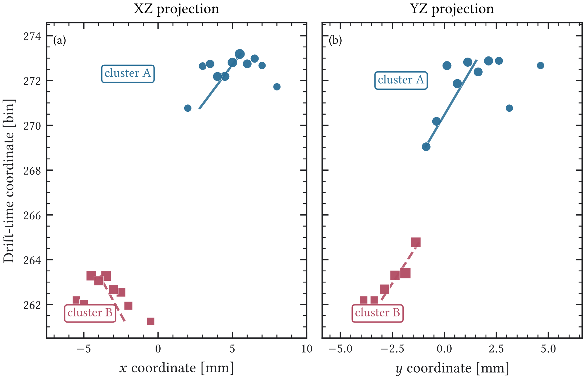
A.1.2 Detector-response parameterization
The gas and veto visible-energy corrections are applied before channel projection and digitization. The physical response model and the approximation implemented in the historical response chain must be distinguished. For a self-recoil in an elemental medium with initial kinetic energy , the conventional Lindhard-type electronic-energy fraction is
(A.1)
with
(A.2)
where is in keV and and describe the target isotope [113]. The electronic-energy fraction includes excitation as well as ionization; its identification with the measured charge yield is an approximation for the present gas mixtures. Gas ionization yields depend on the ion species, energy and corresponding -values, as well as mixture effects [135].
The inspected TRestGeant4QuenchingProcess implementation applies this factor to each deposited-energy hit carrying a hadronic target isotope. That selection does not follow all ionization deposits along an explicitly transported recoil-ion track, and its argument is the individual deposit rather than the recoil’s initial kinetic energy. In general, . The historical implementation therefore is not a validated complete-recoil ionization model.
For scintillator deposits, the first-order Birks approximation is
(A.3)
with a configurable nominal value [109, 110, 136, 137]. Here should be the physical path associated with the deposit. The expression gives a light-yield proxy in the low-stopping-power normalization; comparison with the measured muon-equivalent energy scale also requires applying the same calibration convention to each response variant. The historical process instead estimates it from the shorter distance to a neighboring stored point in the same volume, using a fallback when a suitable distance is unavailable. This chord can belong to the following segment and need not equal the true Geant4 step length. Photon-track local deposits are left unquenched, which also makes the result sensitive to the production-cut treatment of unresolved secondary electrons.
A deterministic two-step check illustrates the effect without assigning a correction to the production samples. Deposits of and over true steps of and give visible energy with the stated Birks constant; the neighboring-point estimate gives , a difference in this constructed example. Splitting a segment at constant stopping power leaves the true-step calculation unchanged, whereas independently applying the integrated Lindhard expression to smaller deposits changes the predicted recoil yield. These algebraic checks identify a segmentation dependence; they do not replace a transport test with recorded true steps, initial recoil energies and nonionizing losses.
The nominal Birks constant is not a dedicated calibration of the BabyIAXO bars: for comparison, a BC408 measurement gives [137]. The historical neutron diagnostic reduces the inclusive energy-weighted gas and veto signals by approximately and , respectively. These inclusive ratios do not bound the effect on low-energy recoil candidates or panel-threshold efficiency. Campaign-specific response versions must be recovered before applying a revised model to an archived background result.
For a veto hit at distance from the effective readout end, the response applies
(A.4)
The current analysis configuration uses an effective attenuation length of ; this is consistent with the approximately factor-two response decrease over a prototype bar, for which [17]. The manufacturer-scale material value of approximately is a different quantity; archived campaigns retain their own recorded response parameters. This effective treatment absorbs reflections, surface finish, optical coupling, and channel-to-channel gain into calibrated parameters rather than tracking optical photons explicitly.
TPC diffusion uses gas metadata derived with Garfield++/Magboltz. A hit of energy is converted to an effective primary-electron population , with optional Poisson or Fano fluctuations, and the electron positions are broadened according to
(A.5)
An empirical detector-hit smearing is applied separately from diffusion to reproduce the measured calibration width and residual gain, avalanche, electronics, and calibration effects. The subsequent raw-signal conversion uses 512-bin waveforms, subsystem-specific sampling and shaping, the peak as the Micromegas energy anchor, and the measured through-going-muon response as the module-dependent veto anchor.
A.1.3 Source normalization and statistical intervals
For an equal-weight source stratum with an ordinary selected count, the central 90% Garwood confidence interval is propagated through the same activity, exposure, energy-window, and fiducial-area normalization as the nominal background level [114, 115]. Rows with , 1, or 2 survivors are instead quoted as one-sided 90% confidence bounds,
(A.6)
in equivalent selected events. The bound is converted to a background level with the same physical normalization as the corresponding sample. This count-dependent choice is a table-reporting convention, not a single interval procedure with guaranteed 90% coverage over all possible observations. For a budget decision or a combined upper bound, a one-sided construction is fixed in advance and applied at every count, or a unified interval procedure with verified coverage is used.
For a source assembled from differently normalized strata, let convert the selected mean count in stratum to its background level, so that . For fixed, independent Poisson samples, a combined interval can be constructed from the joint likelihood , with source and response uncertainties included as nuisance parameters [52]. When an explicitly conservative simultaneous upper bound is required, tail probabilities may instead be assigned in advance with . Summing the corresponding normalized one-sided bounds then gives at least 90% simultaneous coverage by the union bound, provided the marginal constructions are valid. Simply adding marginal 90% endpoints does not establish that statement.
A Garwood interval on the unweighted total count is not exact for an unequal-weight mixture. Correlated descendants, shower particles, and repeated response realizations are grouped by their independent parent history; their multiplicity does not supply independent Poisson trials. For such samples, uncertainty must follow the per-history response estimator or a validated sampling construction. Finite Monte Carlo uncertainty is reported separately from source activity, angular-spectrum, and detector-response systematics. Where a legacy table does not preserve the required strata, its interval is marked as approximate and the row remains auxiliary. Mutually exclusive source scenarios are also kept separate: atmospheric and low-radioactivity argon are alternatives, as are a full HENSA neutron field and a decomposition that uses CRY plus the HENSA-minus-CRY residual. An aggregate HENSA row is not combined with its own prompt and delayed subchannels.
For an equal-weight rare-event endpoint with at most one count per independent history, zero selected events give the Poisson-approximation one-sided bound
(A.7)
This expression is useful for planning exposure only after the source rate and selection denominator have been validated. For exactly independent generated histories with Bernoulli acceptance, the corresponding exact bound is , with its large- limit. With and , a zero-count bound of requires approximately of equivalent exposure. It is not a compute-time estimate, and it cannot be applied unchanged to an all-zero sample with unrestricted descendant multiplicity or unequal weights. The evaluation exposure or a statistically valid stopping rule is fixed before the final sample is inspected; selection optimization uses separate histories.
A.1.4 Reconstruction chain and reference samples
| Analysis stage | Processes in the final configuration | Role in the reconstructed observable space |
|---|---|---|
| Simulation truth and conversion | Geant4QuenchingProcess, Geant4AnalysisProcess, Geant4ToDetectorHitsProcess | Apply the Geant4-stage visible-energy correction, store truth diagnostics for validation, and map Geant4 deposits into detector-hit objects. The truth observables are not used for the final selection. |
| Detector-response emulation | DetectorLightAttenuationProcess, DetectorHitsRotationProcess (before), DetectorElectronDiffusionProcess, DetectorHitsSmearingProcess, DetectorHitsReadoutAnalysisProcess (before) | Model light losses, coordinate alignment, charge diffusion, finite resolution, and pre-digitization readout-plane quantities. |
| Digitization and response calibration | DetectorHitsToSignalProcess, DetectorSignalToRawSignalProcess | Convert detector hits into strip and veto waveforms with the chosen shaping, sampling, trigger delay, dynamic range, and TPC/veto calibration factors. |
| Experimental DAQ input | RawMultiFEMINOSToSignalProcess, RawFeminosRootToSignalProcess | Provide the measured-data entry points before joining the common raw-waveform reconstruction chain. |
| Readout metadata and channel masking | RawReadoutMetadataProcess,RawSignalRemoveChannelsProcess | Attach the detector-channel mapping and remove inactive or noisy channels before waveform analysis. |
| Raw waveform conditioning | RawSignalRangeReductionProcess, RawBaseLineCorrectionProcess, RawCommonNoiseReductionProcess | Emulate the finite ADC range for simulation and apply baseline and common-noise corrections to TPC and veto channels. |
| Raw waveform observables and peaks | RawSignalChannelActivityProcess, RawSignalAnalysisProcess, RawPeaksFinderProcess | Extract channel activity, amplitudes, integrals, threshold observables, peak times, peak multiplicities, and veto-channel information. |
| Signal and hit reconstruction | RawToDetectorSignalProcess, DetectorSignalChannelActivityProcess, DetectorSignalToHitsProcess | Recover detector signals and convert them into reconstructed spatial hits. |
| Reconstructed-hit observables | DetectorHitsReadoutAnalysisProcess (after), DetectorHitsAnalysisProcess, DetectorHitsGaussAnalysisProcess, DetectorHitsRotationProcess (after) | Fill readout-plane, spatial, and Gaussian-width observables after the experimental-like reconstruction. |
| Track observables | DetectorHitsToTrackProcess, Track2DAnalysisProcess | Build the track representation and compute the two-dimensional topological variables entering the X-ray-like selection. |
REST-for-Physics process groups used in the target analysis configuration. The TRest class prefix is omitted in the process column for readability. Simulation-only and experimental-input branches are shown together because both are projected into the same reconstructed observable space before the candidate selection.| Sample | Role | Monte Carlo configuration | Use in the analysis |
|---|---|---|---|
| calibration | Detector-response validation at | Point-like X-ray source, gas matched to the target background sample, chamber-focused geometry | Energy calibration, peak shape, response comparison with calibration data |
| Uniform 0–12 keV gamma | Signal-like acceptance across the low-energy region | Flat low-energy photon spectrum, same gas and reconstruction chain as the calibration sample | Full efficiency versus true incident energy, provided generated photons and reconstruction failures remain in the denominator; otherwise conditional topology response versus reconstructed energy |
| Background source samples | Source-specific residual background | Cosmic, environmental, radon, and contamination sources in the relevant detector geometries | Raw and cut-surviving background populations to be multiplied by source normalizations |
| Experimental calibration data | Empirical accidental veto model | Real calibration events with no physical correlation to simulated X-ray photons | Veto-noise overlay and accidental signal-loss estimate |
A.1.5 Classifier observables and validation
A.1.5.1 Frozen candidate and comparator definitions
The frozen background-analysis-v1 selector uses the primary random seed 1337; two additional seeds are retained only as robustness checks. It is implemented with the HistGradientBoostingClassifier in scikit-learn [138]. For reconstructed topology vector , the ordering score is
(A.8)
as returned by the classifier probability estimator. The value is not interpreted as an absolute physical probability because it depends on the training mixture and class weighting. The frozen topology cut is , with fixed on a signal partition disjoint from model fitting to retain 80% of simulated . During grouped cosmic cross-fitting, no production file is scored by a model trained on that file.
The transparent histogram comparator is a binned signal-to-background log-likelihood ratio. For class , feature , and bin ,
(A.9)
The preserved comparison uses equal-width bins between the pooled finite 0.1 and 99.9 percentiles, edge assignment outside that range, and pseudocount . A larger value is more signal-like, and the comparison threshold is set to 80% validation- acceptance. This definition is related to, but not identical to, the earlier REST-native TRestDataSetOdds workflow, which constructs calibration-only marginal densities and uses the opposite score convention.
The bounded repair study also uses calibration-anchored logistic and robust-distance candidates. For the logistic candidate,
(A.10)
where contains the nearest-calibration median/IQR-anchored and standardized reconstructed features. The signal-only L1 candidate uses the negative mean absolute standardized distance from the calibration center, while the five-feature box uses the negative maximum standardized deviation. The exact run assignments, threshold samples, exclusions, and unopened blind block are recorded in the validation tables below.
| Feature group and derived analysis inputs | Physical interpretation and role |
|---|---|
Hit multiplicity
| Primary separation. Strip-view hit counts expressed directly and through symmetric summaries. Extended or poorly matched tracks tend to activate more strips or exhibit a large view imbalance. |
Charge-cloud size
| Primary separation. Widths of the reconstructed charge distribution in the two strip projections and drift coordinate, together with deterministic transverse summaries. Compact X-ray conversions should be narrow. |
Projection shape and symmetry
| Supporting separation. Disagreement between transverse widths and non-Gaussian asymmetry of the reconstructed charge cloud test whether the two views describe one compact conversion. |
Energy sharing and balance
| Supporting consistency, with one inactive field. Projection-energy balance tests agreement between views. The dominant-track fraction is retained in the frozen contract because it can identify fragmentation before the one-track gate, but it equals unity for every finite event in the evaluated candidate-v1 samples and supplies no separation here. |
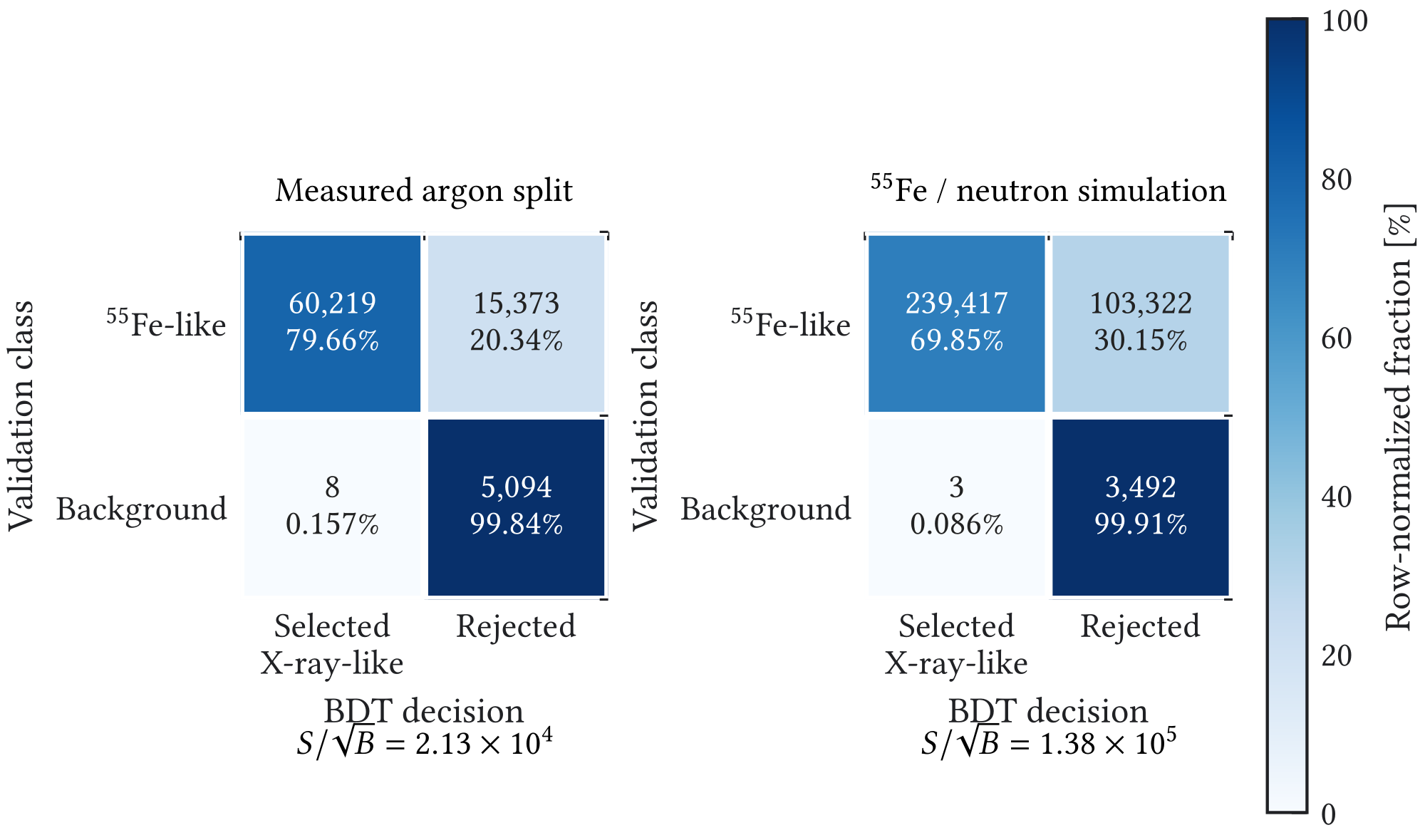
TRestAnalysisTree analysis export, rather than literal ROOT branch names. The calibrated maximum-track energy defines the – analysis window but is not used as a classifier input.| Selector | eff. | kept | acc. | |
|---|---|---|---|---|
| Measured argon calibration/background split | ||||
| BDT, max. | 8/5102 | |||
| BDT, ref. | 9/5102 | |||
| Binned log-odds, ref. | 10/5102 | |||
| Manual cuts | 16/5102 | |||
| Adaptive intervals | 29/5102 | |||
| Gas-matched /cosmic-neutron simulation | ||||
| BDT, max. | 3/3495 | |||
| BDT, ref. | 7/3495 | |||
| Binned log-odds, ref. | 38/3495 | |||
| Simple X-ray cuts | 53/3495 | |||
| Experimental evaluation | Independent result and interpretation |
|---|---|
| Earlier event-random development split, BDT at reference | Calibration: . Background: . Interpretation: Useful selector-development result, but events from the same operating period can occur in both partitions and the preselection differs from the candidate-v1 contract. |
| Untouched August–September run block, calibration-anchored BDT, primary seed | Calibration: , C.I. –. Background: , C.I. –. Interpretation: Threshold fitted only on a disjoint July validation block. Features are robustly referenced to the nearest operational calibration run. |
| Untouched August–September run block, fixed simulation-derived intervals | Calibration: . Background: . Interpretation: Transparent reference; lower background acceptance is accompanied by substantially lower and unmatched signal acceptance. |
background-analysis-v1 check | Result | Consequence |
|---|---|---|
| Cosmic train/evaluation production-group overlap | 0 groups | Leakage condition satisfied. |
| Untouched simulated test | Simulated efficiency gate satisfied. | |
| Measured R02756 domain check | Simulation-to-data efficiency gate failed. | |
| Finite-feature fiducial cosmic candidates | pass topology | Honest cross-fitted diagnostic; not a validated background acceptance. |
| Aggregate HENSA after topology and veto | events, | Replaces the training-contaminated diagnostic -event value, but cannot form the prompt/delayed budget split without history labels. |
A.1.5.2 Bounded 2025 repair-study audit
The bounded repair study was defined only after candidate-v1 failed. R02905 provided a stable calibration reference at an approximately 1.3% peak span. R02997 was retained for threshold setting with a declared 9.9% gain-drift flag, and the shorter R02998 calibration run was retained for non-blind validation with an approximately 4.5% peak span. The originally proposed background runs R03020–R03022 were excluded before model development because they contained one event, only approximately 10 seconds of data, and an anomalous high-rate or incomplete analysis, respectively. The non-overlapping R02993 and R02994 files supplied the 83 non-blind background candidates reported in Table 3.4.
The long R03015 background run and R03018 calibration run were reserved as the final blind block. R03018 carries predeclared gain-drift and spatial-support flags, but neither candidate scores nor acceptances were inspected. The failed non-blind result records selected_candidate=null and blind_input_opened=false; no retuning followed. Thus, the unopened block remains available for any genuinely new, predeclared detector-condition-aware selector.
A.1.5.3 Frozen candidate-v1 transfer diagnostics
The main chapter retains only the score-transfer figure needed to decide whether candidate-v1 can be promoted. The feature-level distributions and model-behavior diagnostics are collected here for reproducibility. R02756 is not used to refit the model or reset its threshold; whenever a score or response surface is shown, it remains the frozen simulation-trained candidate. None of these panels represents an experimental production selection.
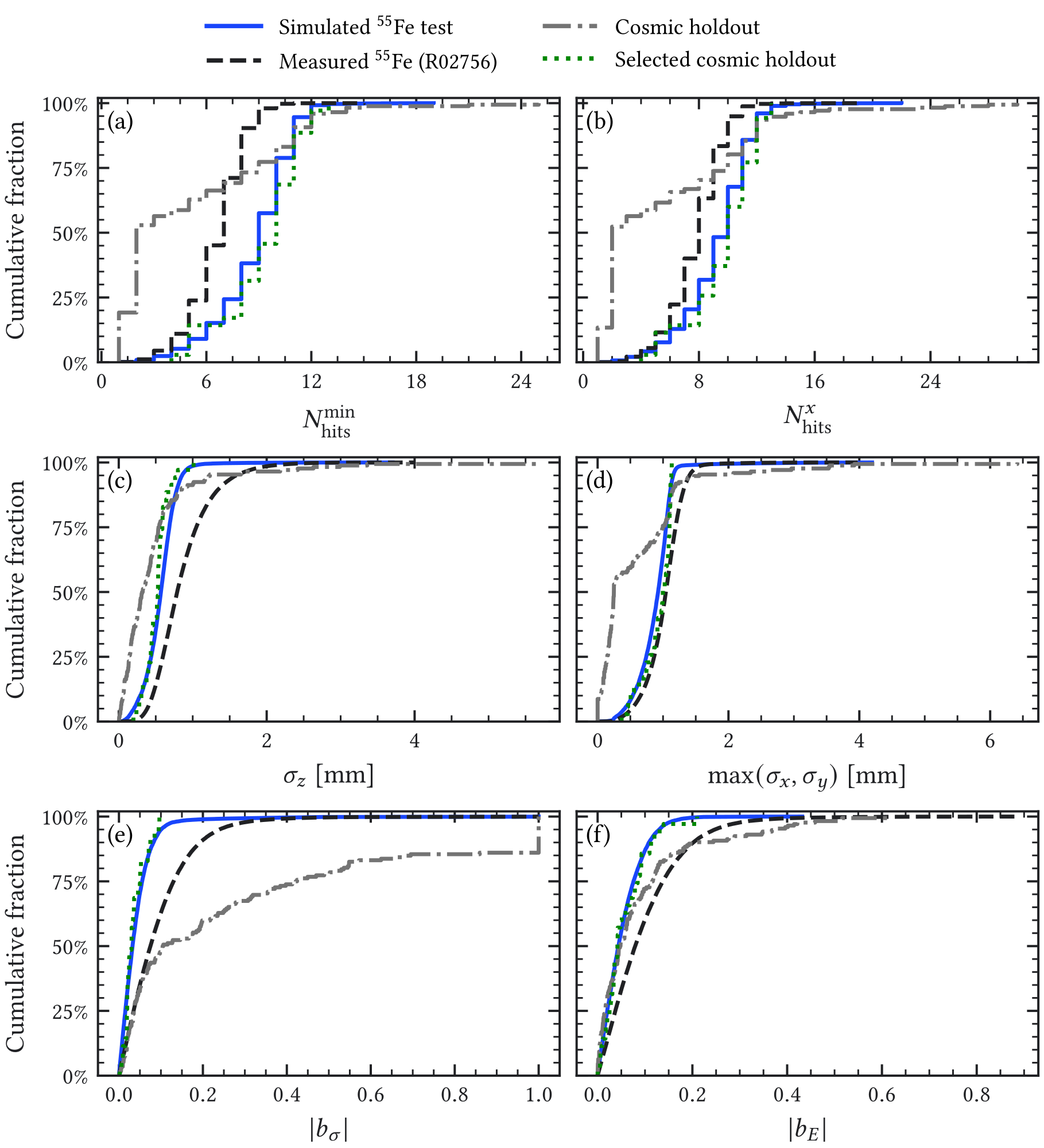
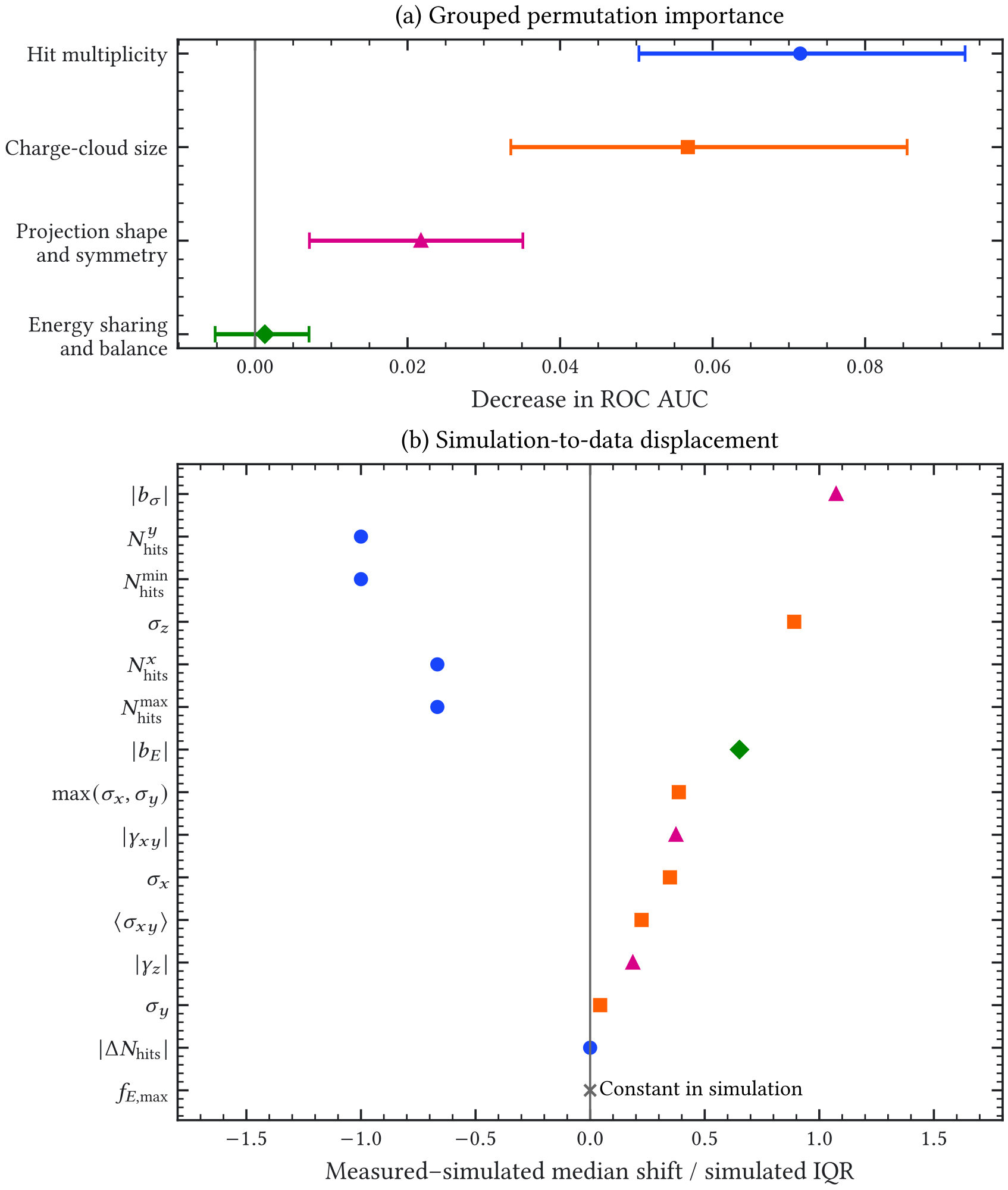
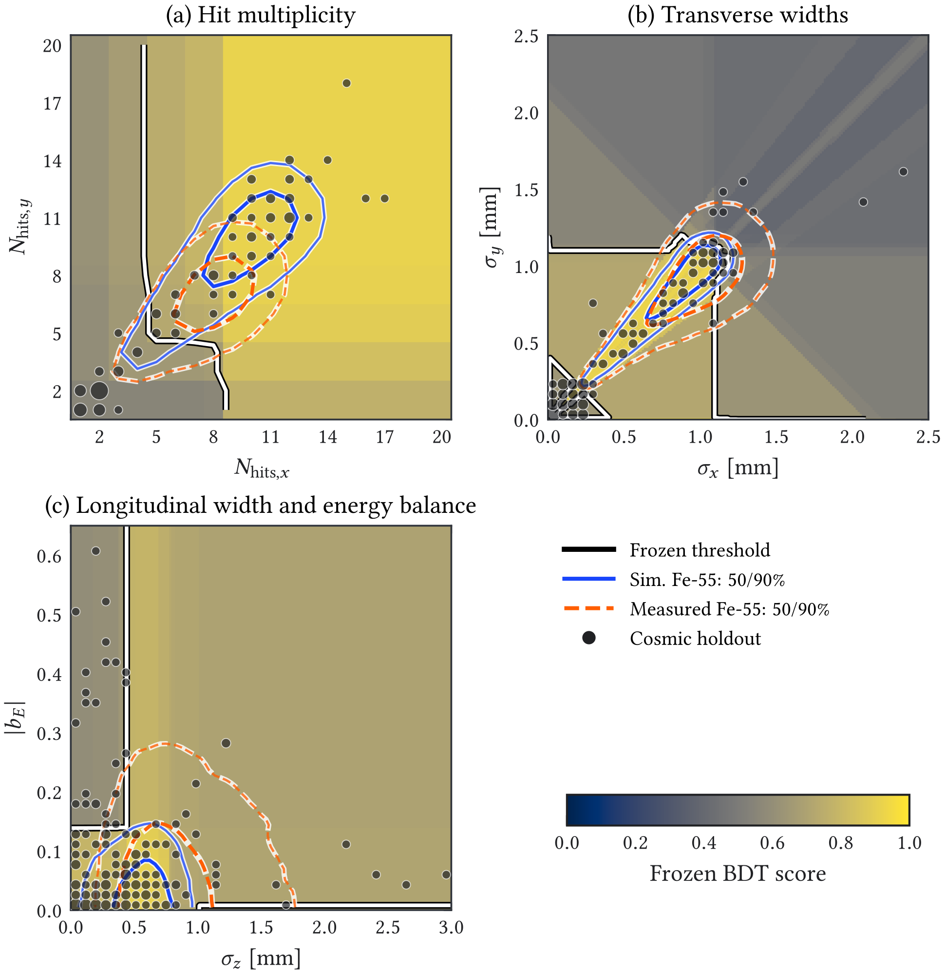
Figure A.7 tests model reliance and detector-domain stability together. Joint permutation keeps deterministically related width and hit summaries in the same feature family. The hit and charge-cloud families that provide most of the simulated separation also exhibit substantial shifts in measured calibration data. The energy-fraction field is constant after preselection.
The response slices in Figure A.8 vary primitive reconstructed quantities, recompute every deterministically dependent summary, and fix only unrelated inputs to a stated reference point. This avoids the impossible feature combinations produced by independently varying a primitive observable and its derived min/max, mean, or balance fields.
A.1.5.4 Historical selector-development and detector-response diagnostics
The figures in this subsection preserve the visual diagnostics that motivated the multivariate study but do not describe the frozen candidate-v1 deployment model. The first two use historical feature sets and development partitions, while the third is a one-dimensional detector-response comparison without a background population.
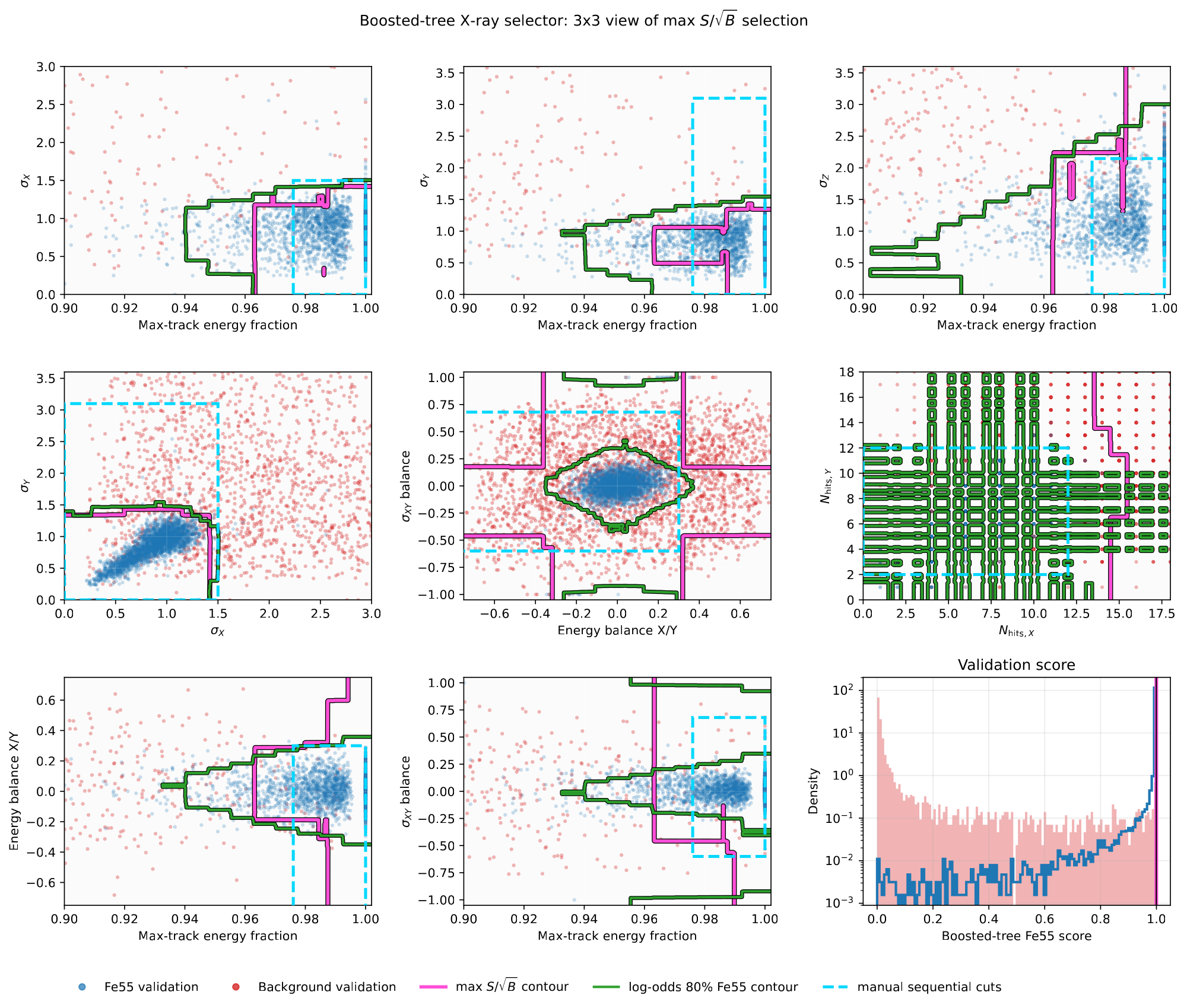
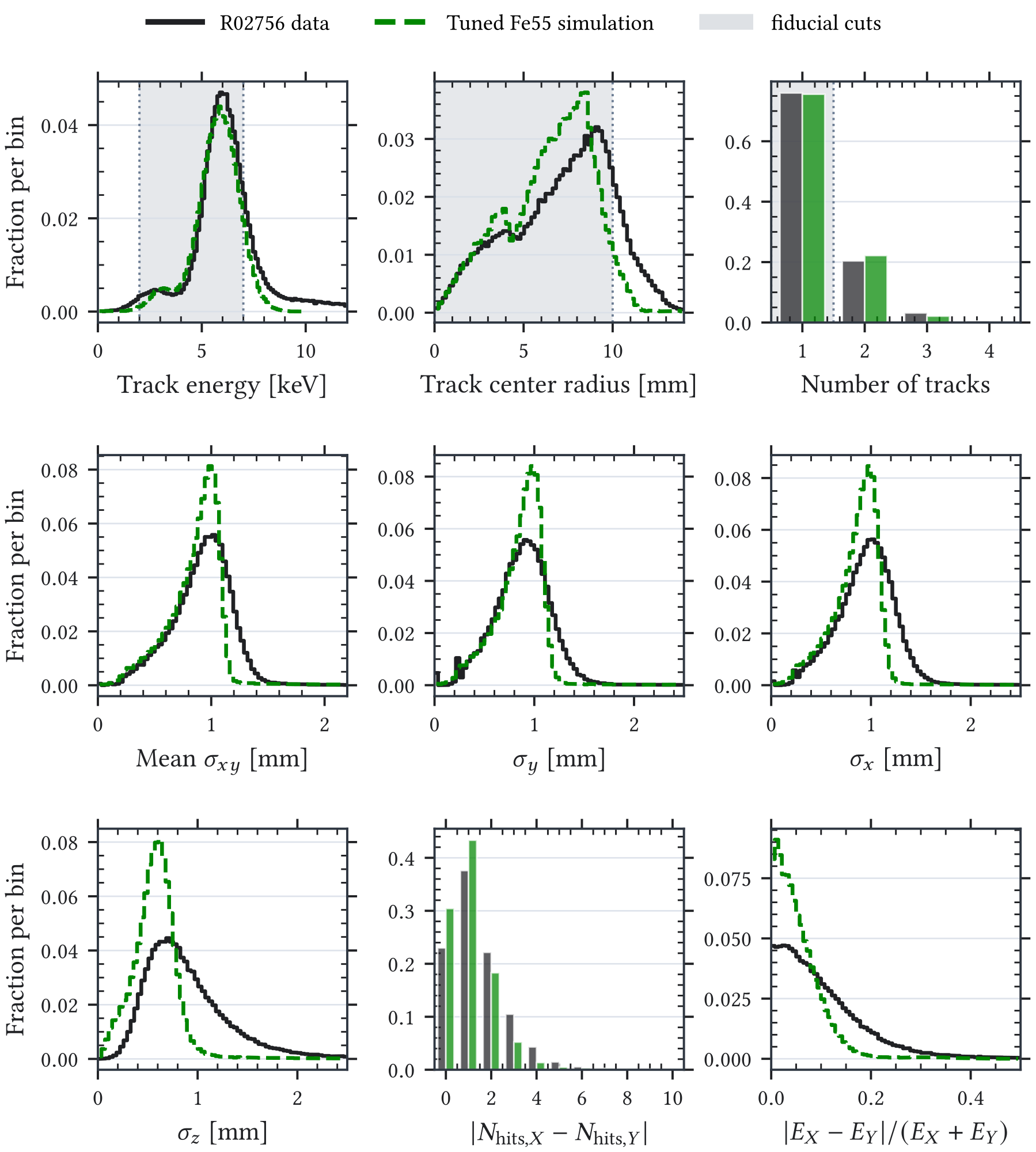
REST-for-Physics analysis chain, and the energy observable is aligned to the calibration peak in each sample. This matrix is retained as detector-response provenance; it contains no cosmic-background population and does not by itself validate the multivariate selector.A.1.6 Legacy candidate-v1 response
A conditional topology response may be reported versus reconstructed energy as
(A.11)
The reconstructed-energy cut is not applied again within a bin already conditioned on . The fixed-retained campaign supplies this conditional response, whereas the companion saveAllEvents production retains the primary energy and failed-reconstruction denominator required for the incident-energy efficiency of Equation (3.2). True-energy weights may be applied to a specified axion spectrum only after the source acceptance, detector-response envelope, and selector validation are fixed.
| Reconstructed energy [keV] | Finite fiducial | Pass topology | Conditional topology efficiency [%] |
|---|---|---|---|
| 2.0–2.5 | 40581 | 11739 | |
| 2.5–3.0 | 42121 | 17416 | |
| 3.0–3.5 | 44265 | 23589 | |
| 3.5–4.0 | 46351 | 28735 | |
| 4.0–4.5 | 47202 | 32418 | |
| 4.5–5.0 | 46384 | 33808 | |
| 5.0–5.5 | 44536 | 33857 | |
| 5.5–6.0 | 41873 | 33061 | |
| 6.0–6.5 | 38731 | 31054 | |
| 6.5–7.0 | 36014 | 29322 |
| True incident energy [keV] | Generated | Pass Micromegas chain | Incident-chain efficiency [%] |
|---|---|---|---|
| 2.0–2.5 | 41885 | 1943 | |
| 2.5–3.0 | 41726 | 3290 | |
| 3.0–3.5 | 41801 | 5525 | |
| 3.5–4.0 | 41561 | 7525 | |
| 4.0–4.5 | 41497 | 8710 | |
| 4.5–5.0 | 41531 | 9186 | |
| 5.0–5.5 | 41912 | 9440 | |
| 5.5–6.0 | 41754 | 8684 | |
| 6.0–6.5 | 41712 | 7302 | |
| 6.5–7.0 | 41712 | 5128 |
A.1.7 Calibration and run-catalog diagnostics
The calibration plot in Figure A.12 is kept here as provenance for the track-energy observable used in the manual and machine-learning X-ray selections.
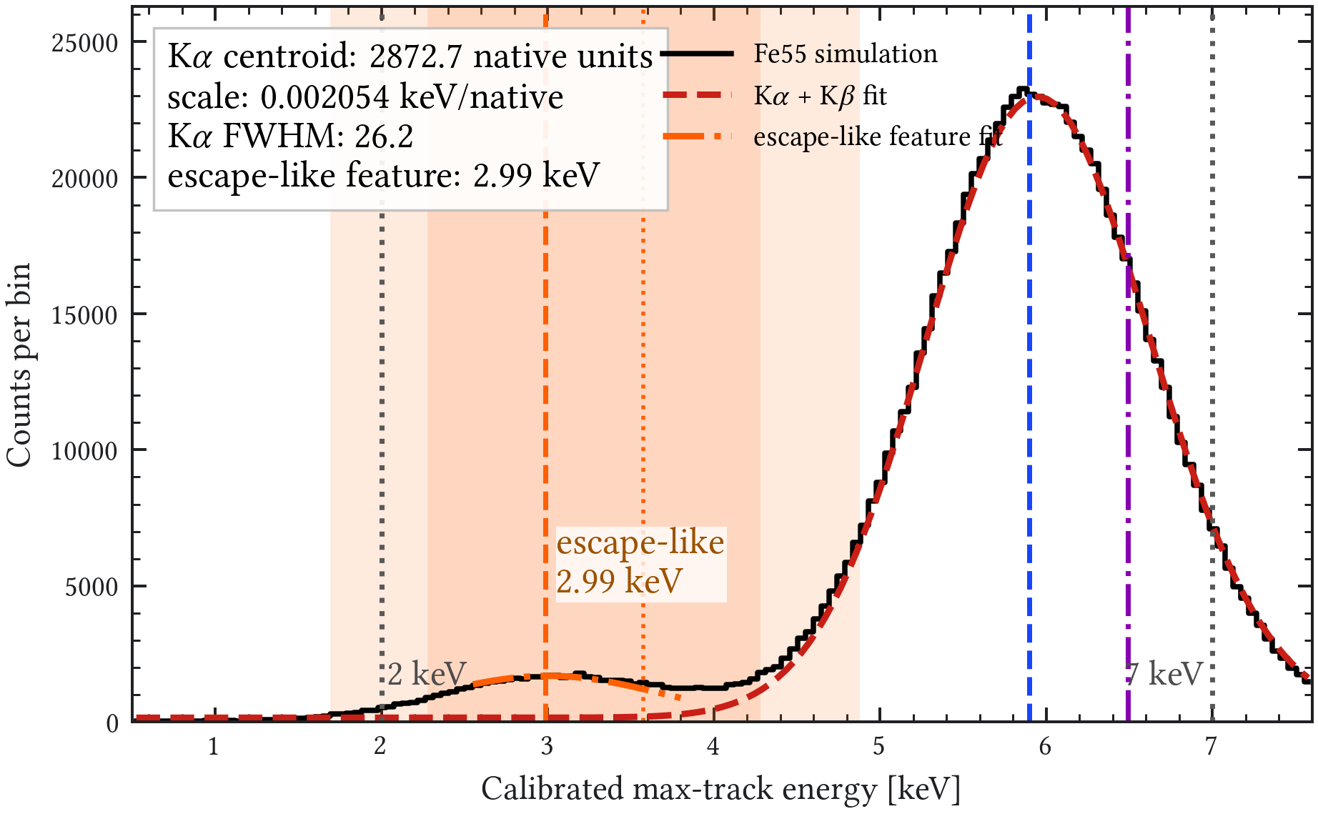
The IAXO-D0/D1 experimental calibration catalog is also kept as a run-level diagnostic. Figure A.13 shows the -candidate runs between May and December 2025 for the argon–isobutane 1% and 2% mixtures. It is not used as a detector-performance average; instead, it documents when comparable calibration files were available and gives the fitted full-model energy resolution for each successful run.
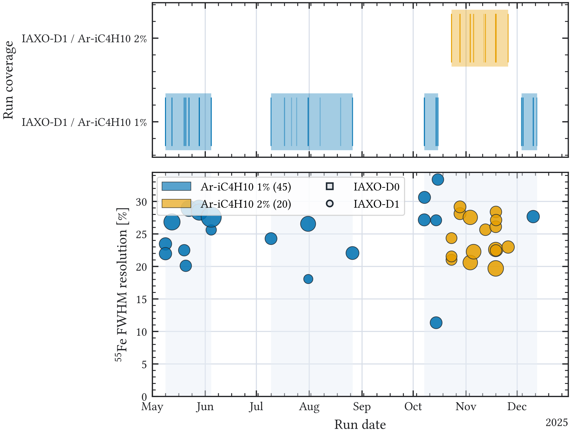
A.2 Supplementary cosmic-veto noise diagnostics
The background-model chapter uses the cosmic-induced visible trigger rate and accidental-coincidence probability as the quantitative veto-noise inputs. The peak-topology and panel-occupancy results collected here are supporting diagnostics of how the reconstructed rawPeaksVETO activity appears in the scintillator system; neither enters the absolute trigger-rate normalization.
The veto activity differs in topology across the primary classes. Figure A.14 summarizes the reconstructed veto-peak multiplicity and the distribution of peak energy within each visible trigger. The left panel shows that muon-induced veto triggers are typically multi-peak events, while gamma-induced triggers are concentrated at one or two peaks. The right panel uses the ratio between the largest reconstructed veto peak and the total reconstructed veto-peak energy as a compact measure of energy concentration. The dashed curve indicates perfectly equal sharing among peaks. All components lie above this line, showing that even multi-peak veto triggers are usually not evenly distributed; one or a few peaks carry a disproportionate fraction of the reconstructed veto energy. The high-multiplicity tail should be interpreted cautiously for low-statistics bins, in particular for gamma events above several veto peaks. No requirement is applied in this diagnostic. The multiplicity axis illustrates the reconstructed activity available to calibrated multivariate selections; it does not define a standalone operational veto criterion.
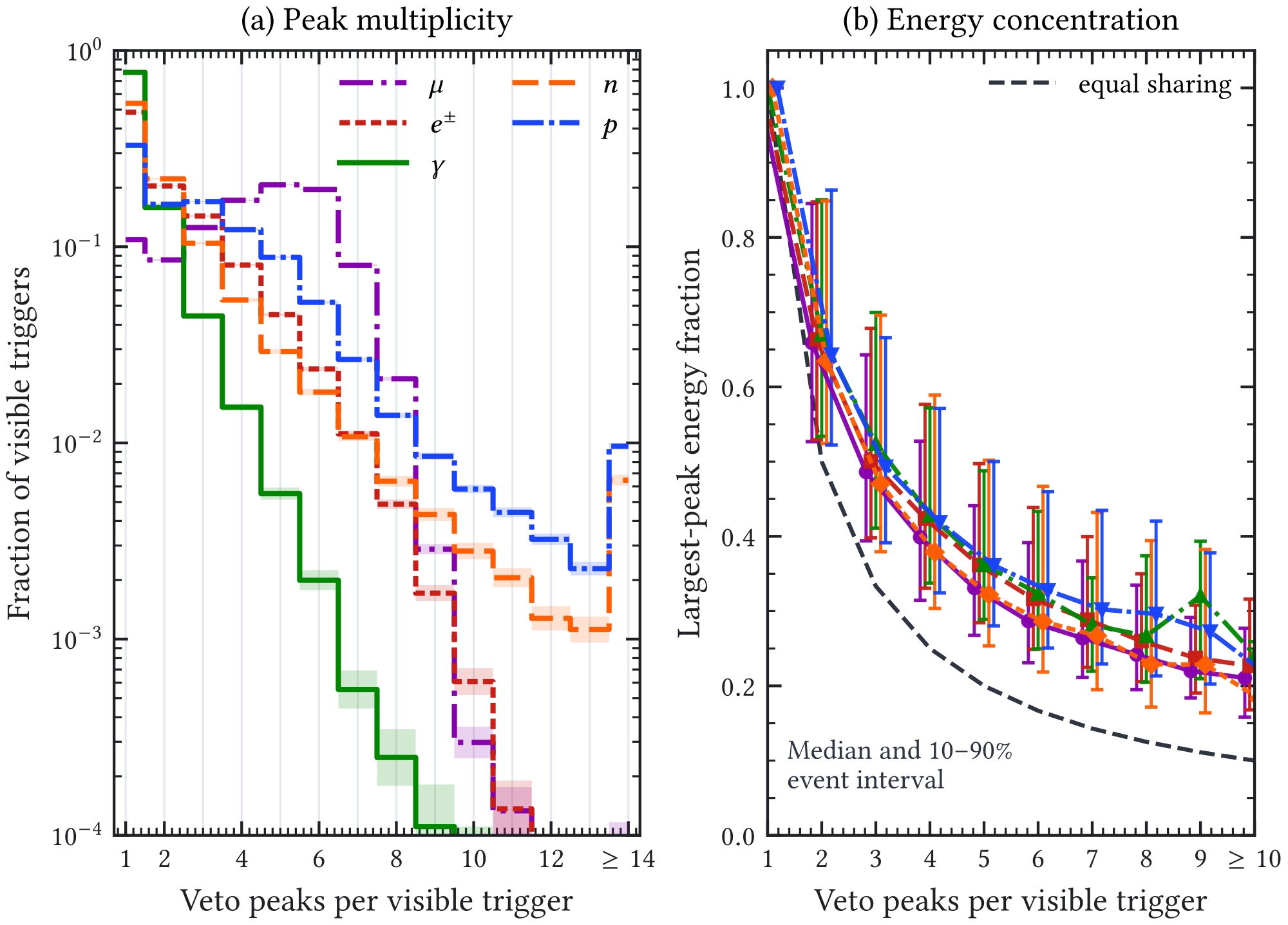
The full coincidence-window dependence is shown in Figure A.15. It treats each visible cosmic event as a Poisson point trigger. A finite correlated peak train changes the effective interval over which any peak can overlap the signal window, so this approximation is not an exact waveform-occupancy calculation. It is not a Micromegas-background rejection curve and not a measured dead-time curve.
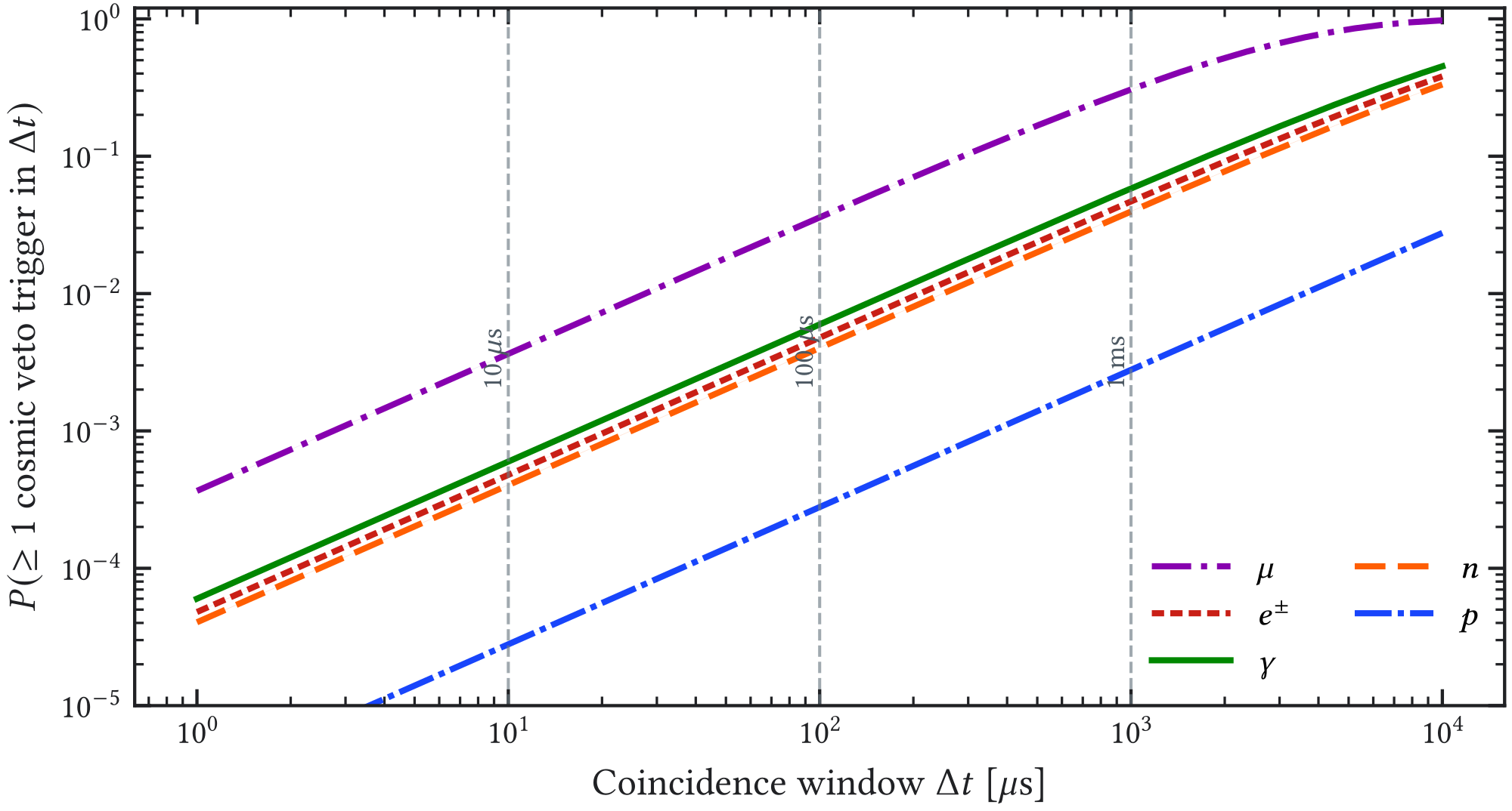
The complementary veto-panel occupancy diagnostic is grouped by veto side and layer. It should be read as a conditional detector-topology plot, not as an absolute trigger-rate plot.
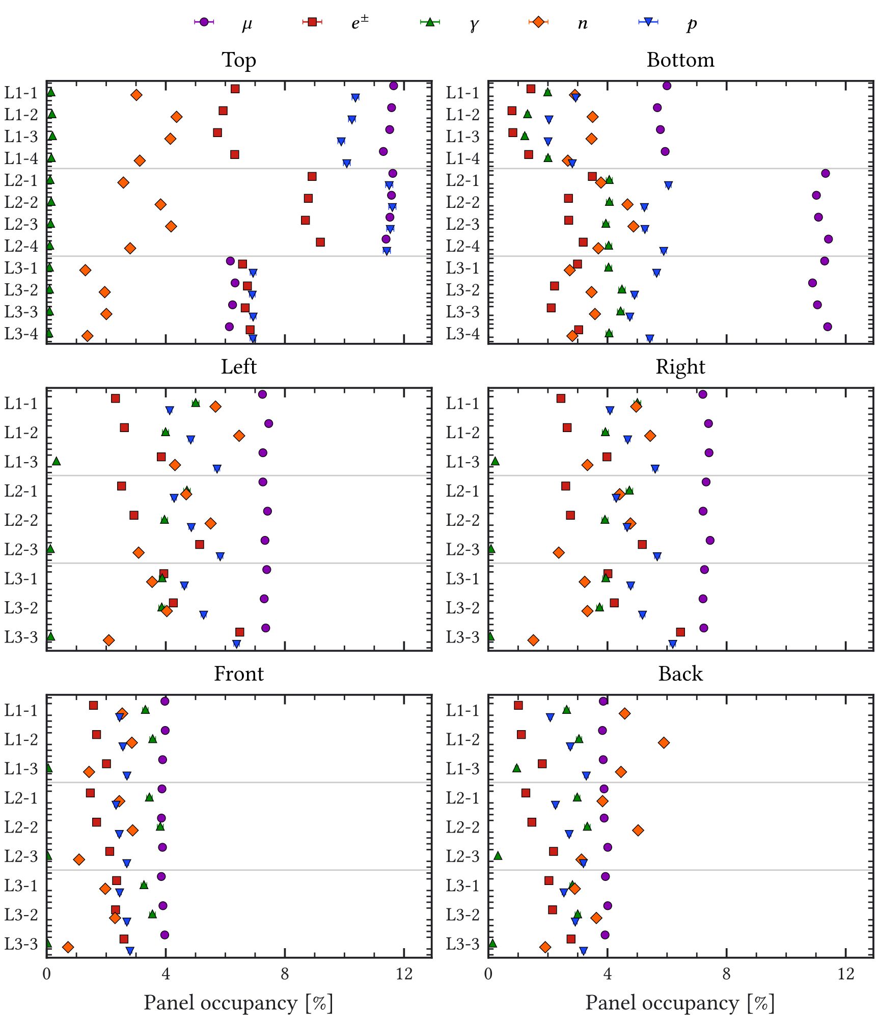
A.3 Supplementary gas and radon contamination diagnostics
The background-model chapter treats gas-borne and radon-related contamination sources as source hypotheses whose absolute rate depends on the gas inventory, gas-handling configuration, and plate-out history. The figures below preserve the diagnostic material used to verify the Geant4 source definitions and the qualitative event topologies. They are kept in the appendix because they support provenance and interpretation, while the main text uses the compact source taxonomy in Table 3.7.
![Figure A.17: Decay chain of 222 Rn , included as reference for the radon and surface-progeny source split used in the intrinsic-background model. Adapted from [ 123 ].](assets/a406e61e12b8506e225123e9.png)
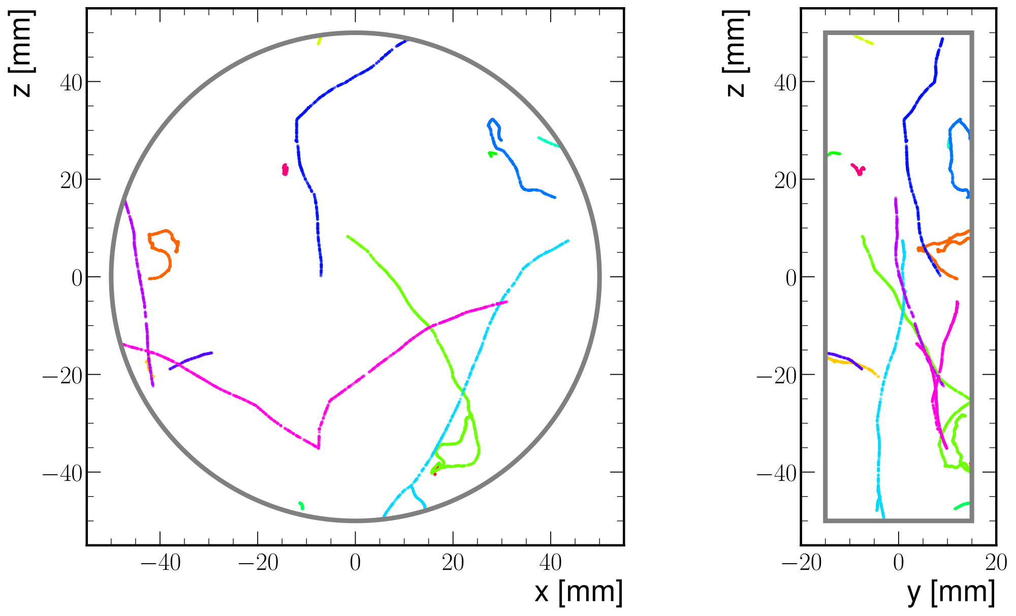
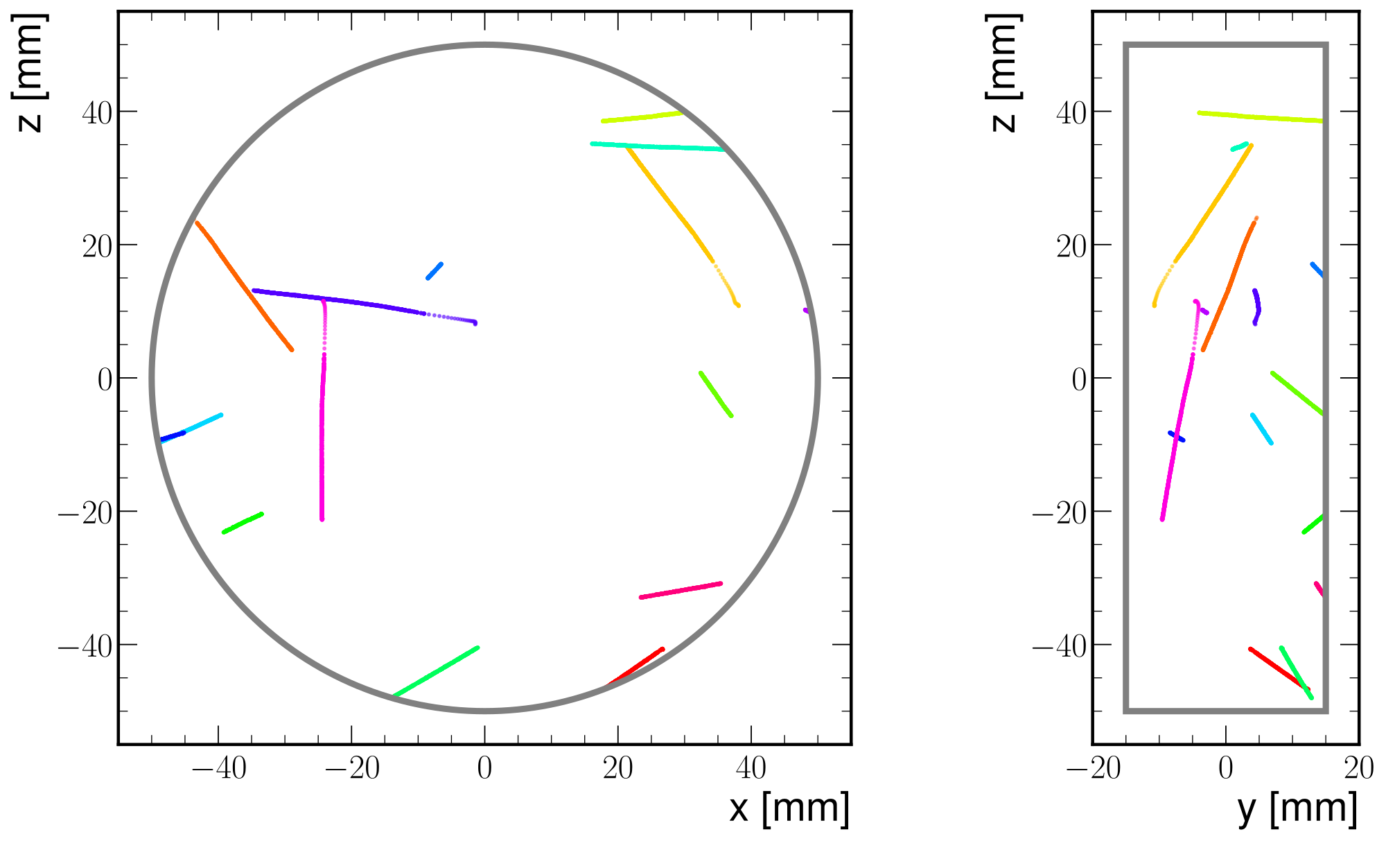
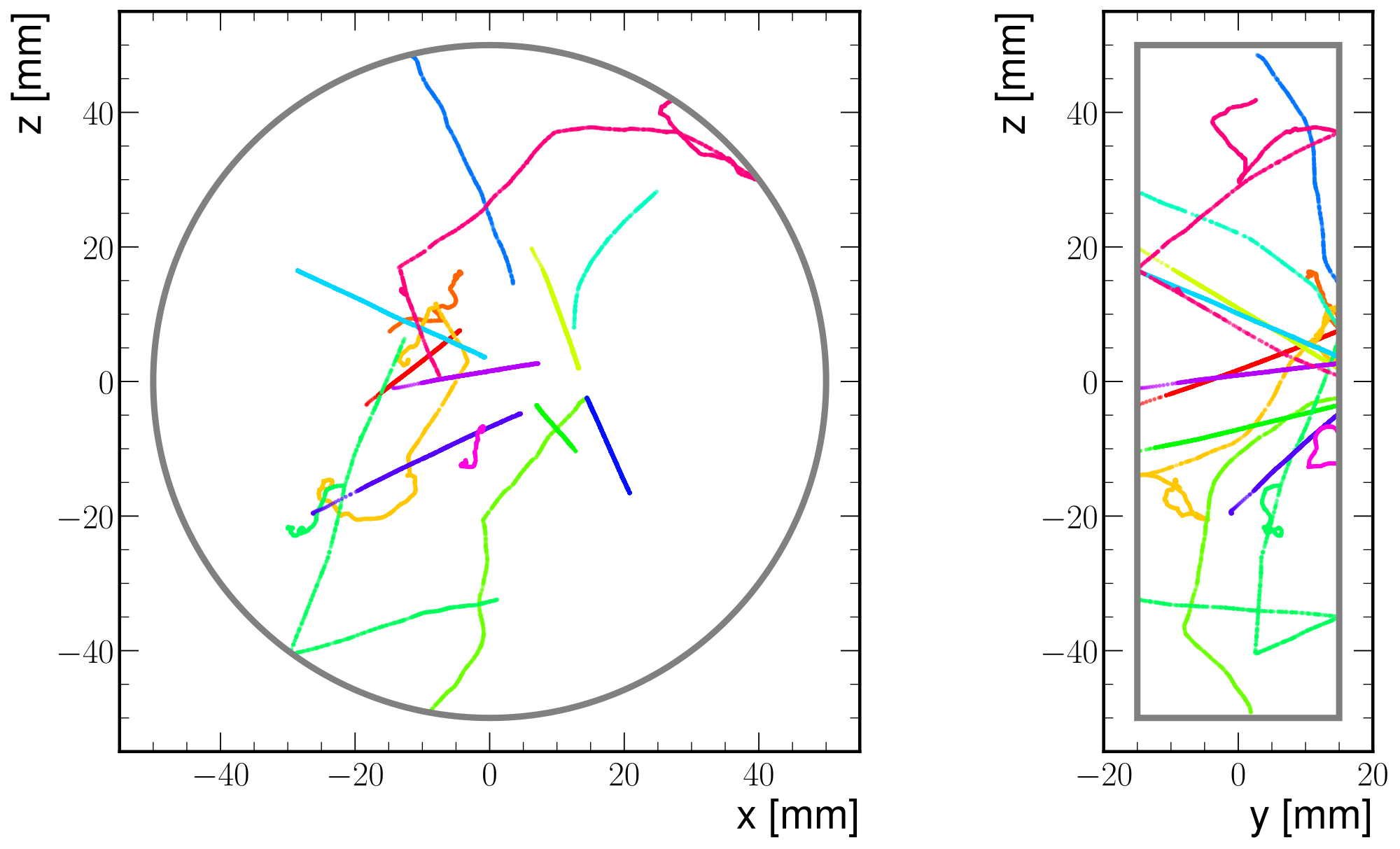
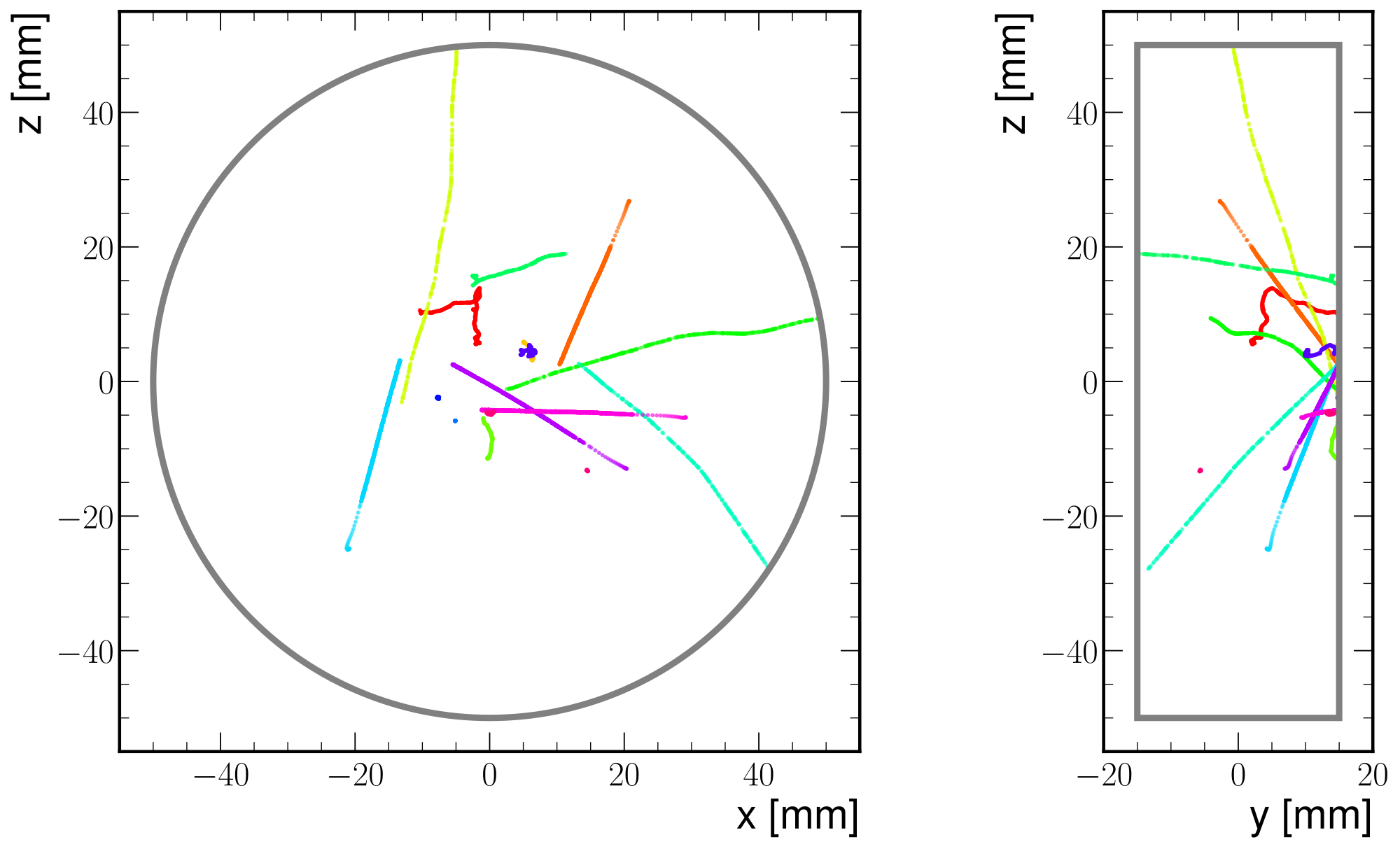
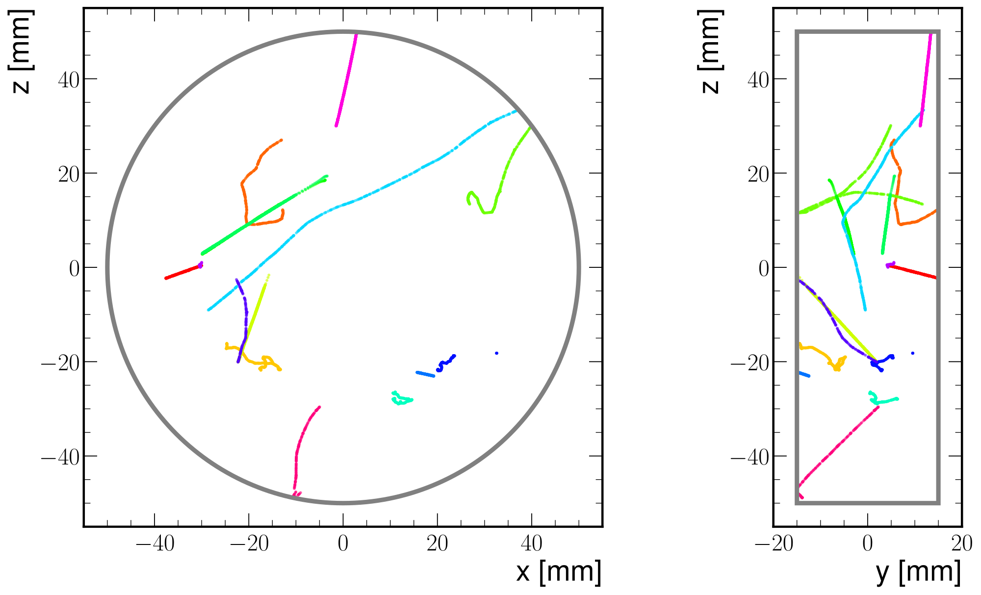
D Ancillary Detector and Calibration Material
A.1 Entrance-window transmission
![Figure A.1: Transmission of low-energy X rays through the aluminized Mylar entrance window, calculated from photon attenuation data [ 68 ]. This signal-region effect belongs to the detector-efficiency model rather than to the veto-rejection mechanism.](assets/51be8c365a11e00eb4c7850a.png)
A.2 Prototype services and AGET/Feminos electronics
The main Micromegas chapter retains the detector requirements imposed by gas handling, high voltage, slow control, and acquisition. This appendix records the implementation details of the IAXO-D0/D1 prototype services and the commissioned IAXO-D0 AGET/Feminos chain.
A.2.1 Gas, high-voltage, and slow-control implementation
The prototype gas line supplies the selected mixture from a high-pressure bottle through pressure reduction and computer-controlled flow and pressure regulation. A vacuum branch permits evacuation during a gas change, while relief valves protect the thin entrance window against excessive differential pressure. The aluminized Mylar window and its copper support were designed for pressure differences up to .
The system can operate in open loop, continuously exhausting the used mixture, or in closed loop with recirculation and purification. Open-loop operation is operationally simple for inexpensive argon mixtures. Closed-loop operation reduces consumption and is more appropriate for xenon–neon mixtures, but requires filtration, recirculation, and continuous monitoring of pressure, flow, oxygen, and moisture. The CAST pathfinder experience showed that this mode is a practical requirement for stable long campaigns with expensive mixtures [80].
Two high-voltage channels bias each Micromegas detector: the cathode establishes the drift field, and the mesh establishes the amplification field. Filtering, controlled ramping, current monitoring, and trip handling are required because discharge behavior and high-voltage noise affect both detector stability and reconstructed pulse morphology. The photomultiplier tubes of the active veto use separate channels, but their gain and timing stability enter the same operational record.
The CAEN supplies can be operated over a serial interface. The hvps library developed in this thesis provides the reusable control backend described in Section 4.7.3. It supports remote monitoring, controlled recovery after short trips, operator alerts, and protective shutdown after repeated trips. These functions are integrated with a Node-RED-based slow-control layer [79], whose dashboard also records gas and environmental conditions.
A.2.2 Commissioned IAXO-D0 acquisition hardware
The IAXO-D0 front-end card contains four AGET (ASIC for Generic Electronics system for TPCs) chips [81]. Each chip provides 64 channels, a 512-sample switched-capacitor buffer, sample rates up to , configurable shaping between and , selectable polarity, four charge ranges, and self-trigger capability. Sixty channels per chip are used for the 240 Micromegas strips.
![Figure A.4: Functional architecture of the AGET front-end chip [ 81 ].](assets/df17ccd8c20240637bee9b20.png)
The front-end card is connected to a Feminos module [75]. Its field-programmable gate array configures the AGET chips, controls timing and readout, and transfers data to the acquisition computer over Gigabit Ethernet. Multiple Feminos modules can share a Trigger Clock Module when synchronous acquisition is required. Configuration commands are sent over the same control link; for example, aget * time 0x1 sets the shaping-time register for all chips, with the physical shaping time determined by the run-specific configuration map.
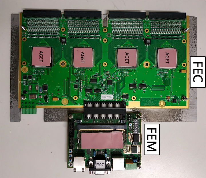
At run start, the acquisition software configures and powers the front end, starts the boards, receives their UDP frames, and constructs the event files with run metadata and channel waveforms. The software refactor, output format, compression, and live monitoring are described in Section 4.7.2. This AGET/Feminos implementation is the commissioned IAXO-D0 reference, not the STAGE/ARC-oriented IAXO-D1 or final BabyIAXO electronics design.
A.3 Supplementary UV-light calibration R&D
During the CEA Saclay internship, a compact Micromegas setup was used to test whether pulsed ultraviolet light could provide a controllable source of photoelectrons for gas-transport and timing studies. The material is kept in the appendix because it is related to detector calibration and Micromegas operation, but it is not part of the baseline BabyIAXO background-model chain. The main text summarizes the methodological relevance of this work in Section 3.6.2.
![Figure A.6: PICOSEC detection concept [ 82 ], included as motivation for the use of ultraviolet photons and a photocathode with a Micromegas amplification structure. A charged particle produces Cherenkov photons in a radiator; the photons release photoelectrons at the photocathode, and the electrons are then drifted and amplified in the Micromegas stages. The CEA internship study used the same general idea of UV-induced photoelectrons, but in a simpler calibration-oriented geometry.](assets/15946d92c884309eb891109b.jpg)