Experimental Typst web edition · Veto chapter pilot
6 Background Model
Introduction
As a rare-event search experiment, IAXO requires a detailed background model to distinguish signal candidates from background events. The purpose of the model is to translate measured activities and external particle fluxes into reconstructed, X-ray-like survivor rates in the Micromegas region of interest. This translation is non-trivial because the same source activity can produce different accepted rates depending on geometry, detector response, selection criteria, veto response, and normalization uncertainty.
In this chapter, the signal reference is a compact X-ray conversion reconstructed in the active gas and within the signal fiducial region. A background component is any other physical source that can produce a reconstructed event compatible with that reference. The model uses the IAXO-D0 surface data as an experimental-validation legacy and IAXO-D1 as its argon–isobutane simulation reference; both are Micromegas prototype configurations that inform, but are not, the BabyIAXO detector. It records for each source component whether transport, reconstruction, normalization, and a compatible detector response are available. The work develops the earlier Micromegas background-model studies documented in the theses of Elisa and Cristina [60, 80], which applied the CAST background methodology to earlier detector configurations. The quantitative endpoint of the chapter is the current partial source-response model for the IAXO-D1 argon–isobutane detector configuration. It uses one deterministic Micromegas reference selection and does not credit an unvalidated topology classifier with background rejection. For components whose absolute activity or site source term is still scenario dependent, the tables separate generated-event yields from auxiliary rate scenarios and identify the source or parent-decay denominator needed for an absolute prediction. The final synthesis combines contract-compatible rows, historical response scales, and an explicit closure matrix, but it does not assign zero contribution to omitted sources or form an arithmetic total from incompatible rows. The BabyIAXO xenon–neon detector, optics acceptance, final veto response, and DESY source terms are treated as separate projections rather than folded into the IAXO-D1 argon reference.
Table 6.1 first fixes the energy windows used when comparing these source components and reference samples.
| Window | Role in this thesis | Usage |
|---|---|---|
| – | Detector-design region | Broad IAXO Micromegas X-ray region used when discussing detector requirements and comparison with earlier Micromegas background goals. |
| – | Simulation diagnostic range | Wide low-energy range used in some source-construction plots to verify spectral shapes, leakage mechanisms, and detector-response behavior. |
| – | Reference analysis window | Default window for the deterministic IAXO-D1 reference selection, the topology-development studies, and comparison with the published IAXO-D0 surface veto analysis. |
6.1 Scope, analysis contract, and claim levels
A source-by-source model is additive only when its source normalizations, reconstructed-event definition, and selection efficiencies refer to the same analysis contract. Sharing an energy interval is not sufficient: changing the energy estimator, fiducial object, topology classifier, veto requirement, or area normalization changes the response factor that multiplies the source activity or flux. This distinction became important during the present work because several historically valid studies used different selections while being described informally as the same “X-ray cuts.”
The final deterministic thesis reference is identified as background-analysis-v2-conservative-reference. Its machine-readable configuration records the detector configuration, branch definitions, event selection, normalization area, interval convention, veto bookkeeping, and explicit prohibition on topology-rejection credit. Table 6.2 gives the physics-level definition needed to interpret the compatible results in this chapter.
| Contract item | Conservative thesis-reference definition |
|---|---|
| Quantitative detector scope | IAXO-D1 with Ar–iCH (1%) at 1.4 bar. BabyIAXO Xe–Ne, optics, final-veto, and DESY-site predictions are separate projections. |
| Reconstructed energy | Calibrated maximum two-dimensional-track energy, tckAna2D_MaxTrack_XZ_YZ_Energy, with the closed interval . The energy is not a classifier input. |
| Track validity | Valid maximum-track reconstruction in the XZ and YZ views, followed by exactly one reconstructed track in each strip projection. |
| Signal fiducial | Maximum-track center , corresponding to . The earlier readout-energy or hit-centroid constructions are auxiliary definitions and are not aliases for this cut. |
| Topology treatment | No learned classifier or additional topology-shape rejection is credited; the deterministic one-track requirement remains part of the response. Candidate-v1 and the bounded v2 family are retained only as diagnostic studies. |
| Veto treatment | The baseline response is reported before veto rejection. A source-appropriate veto stage may be reported separately when the channel is identified: prompt rejection is applied only to prompt events, delayed activation receives no prompt-veto credit, and accidental signal loss or live time is a separate efficiency. |
| Normalization and intervals | The full readout area is used before the fiducial stage and afterward. Rates use the window width. Counts above two receive central Garwood intervals; zero, one, or two survivors receive one-sided Poisson upper bounds. This is a reporting convention; a coverage or decision claim requires one predeclared construction for all counts. |
| Inclusion rule | A row enters the thesis partial reference only if it records this identifier and applies every definition above. No total is formed while physical sources, normalizations, or mutually exclusive scenario choices remain open. |
The deterministic reference is the consequence of two explicit negative validation results, not an assumption that topology carries no information. The frozen candidate-v1 BDT retains of untouched simulated but only of the measured R02756 domain-check sample. A subsequent bounded candidate family reached the nominal calibration working point, but no candidate passed the independent non-blind background-rejection gate. No v2 candidate was selected and the reserved R03018/R03015 blind block was never opened for selector evaluation. The topology studies therefore remain reproducible diagnostics, while the energy, one-track, and fiducial stages define the thesis partial reference.
The source registry assembled for this chapter contains 30 physical source records, in addition to one source-construction diagnostic and two X-ray control samples. Under the conservative reference, four light-cosmic source rows already have a directly usable deterministic response, 11 physical sources have preserved outputs suitable for reference-selection reprocessing, eight are blocked primarily by an absolute normalization, and seven still require a source or geometry definition. Seventeen named physical sources were absent from the illustrative numerical synthesis. These counts provide a completeness statement: they show that a missing row is an open component, not evidence for a zero contribution.
The following status labels are consequently used throughout the chapter and may coexist for a single source. An analysis-contract-compatible result has been evaluated with the complete deterministic definition above. A legacy or auxiliary result is scientifically useful for mechanism or scale but cannot enter the common sum unchanged. A scenario-normalized result has a simulated response but depends on an adopted activity or site source term. An open component still lacks the response, normalization, or both. Only results that are contract-compatible and use mutually consistent source assumptions are eligible for the partial reference; central estimates, one-sided bounds, and open components remain separate in the present synthesis.
6.2 Simulation and analysis methodology
The background model simulations and the subsequent event reconstruction were carried out with REST-for-Physics [83], using the restG4 and restManager applications described in the software chapter. The Monte Carlo transport stage was defined through source-specific configurations, while the detector-response emulation and event reconstruction were performed with a common analysis chain. This same reconstruction chain is also used for the analysis of experimental data, since the simulated detector response is converted into the same reconstructed event format as real detector acquisitions. This common data model allows the same observables, selection criteria, and background-discrimination procedures to be applied consistently to both simulated and measured events.
6.2.1 Workflow overview
The methodology followed for the background model is summarized in Figure 6.1. The first stage consists of defining a source term and the corresponding detector geometry. The source term depends on the origin of the background contribution under study: radioisotope contamination in a detector component, environmental radiation entering from outside the shielding, or cosmic-ray secondaries. These inputs are then propagated with restG4, which performs the Geant4 transport and stores the event-level truth information.
In a second stage, restManager processes the simulated event through a detector-response chain designed to reproduce the experimental readout observables as closely as possible. This response chain includes both the Micromegas detector readout and the active-veto readout, which are described in REST-for-Physics through dedicated readout definitions. Although both systems are handled within the same analysis framework and are ultimately stored in a common event structure, they represent physically different detector subsystems: the Micromegas readout reconstructs the charge signal produced in the gaseous TPC, while the veto readout reconstructs scintillation signals produced in the surrounding veto modules. Consequently, their channel mapping, signal formation, timing, shaping, and reconstructed observables are treated with subsystem-specific parameters and processes.
The reconstructed output is then used to derive the observables employed for the background studies and for the X-ray-like event selection. In this way, the simulated events can be compared with experimental data at the level of reconstructed quantities, rather than only at the level of idealized energy depositions.
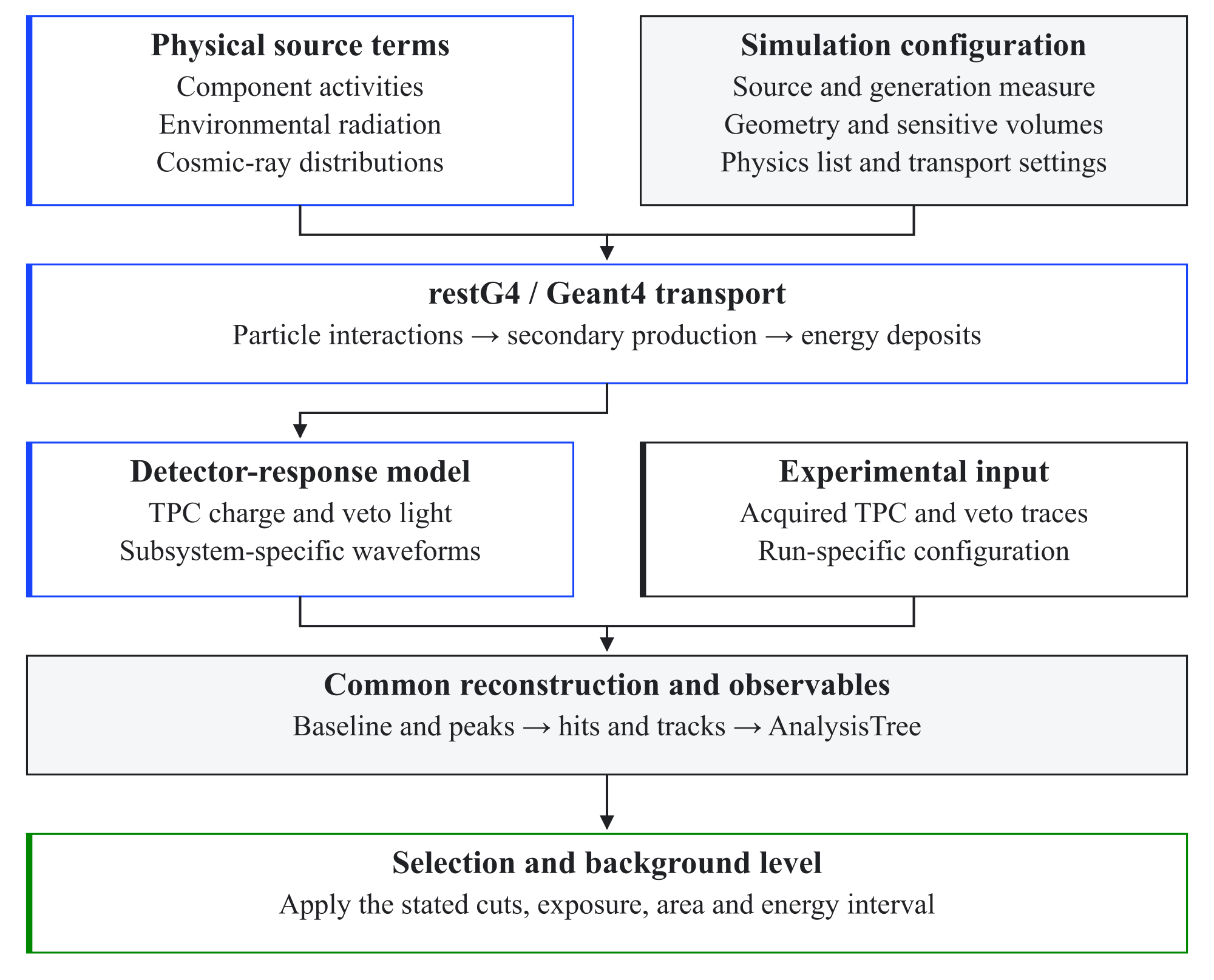
restG4, producing Geant4 truth-level events. The resulting events are then processed with restManager through the detector-response and reconstruction chain. Dedicated REST-for-Physics readout descriptions are used for the two instrumentally different subsystems: the Micromegas TPC readout and the active-veto readout. The final output is a set of reconstructed observables that can be analyzed with the same selection logic used for experimental data.This separation between transport and reconstruction was particularly important in the present work. It allowed the same reconstruction chain to be applied consistently to different background sources, while at the same time making it possible to update detector-response parameters, electronics settings, veto thresholds, or analysis cuts without repeating the full Geant4 transport stage. The same strategy also ensured that simulated events and experimental data were compared using the same reconstructed observables and selection criteria, while preserving the distinct detector-response models required by the Micromegas and veto readout systems.
6.2.2 Source-specific simulations
The Monte Carlo transport stage used a family of source-specific descriptions. Each one defined the source term for one background component, but the structure of the simulations was kept common: a detector geometry, a primary-event generator, the sensitive detector volumes, and the physics lists required for electromagnetic interactions, radioactive decays, and, when needed, hadronic transport. This organization isolates the physical origin of each background contribution while preserving a common interface to the reconstruction chain.
For internal contaminations, the simulated source was defined from the detector volume corresponding to the material under study. This category includes detector materials such as copper, electronics, gas, Kapton, aluminized polyethylene terephthalate (PET; Mylar), shielding elements, and radon or plated-out progeny. The primary positions were sampled uniformly inside the selected volume, or on its surface when the measured contamination was given as a surface activity.
The activity assigned to each source was obtained from radiopurity measurements performed by the collaboration at the Laboratorio Subterráneo de Canfranc. For a mass-specific activity or surface-specific activity , the source normalization is or , respectively, where or is the simulated material mass or surface.
When the measured activity referred to a parent isotope assumed to be in secular equilibrium, the full radioactive decay chain was simulated. In this way, the generated events preserve both the spatial distribution of the contamination in the detector geometry and the correct normalization to the measured activity of the material.
Environmental backgrounds were also considered in the simulation campaign, although their final importance depends on the site-specific radiation field and shielding configuration. At the time when these studies were developed, the experimental layout under consideration assumed that the detector would operate inside a laboratory environment, with at least partial underground overburden. Under those assumptions, radiation from the surrounding laboratory materials, such as concrete gammas and neutrons, was a relevant contribution to evaluate.
These backgrounds were treated as external fluxes incident on the detector and shielding system. When a direct simulation from the laboratory boundaries was inefficient, the source term was factorized into two stages. The calculation first obtained energy and angular distributions for particles emerging from the surrounding materials, then used them as input spectra for the detector-level simulation. This avoided repeating the expensive laboratory-scale transport for each detector-response or selection study.
Under the current outdoor, on-surface BabyIAXO working scenario, cosmic-ray-induced backgrounds are expected to become more prominent than in a deep underground installation. The relative importance of the environmental and intrinsic components cannot nevertheless be ranked until a site-specific source term and conservative-reference responses are available. Nearby telescope structure can also constitute an environmental source term, but its contribution cannot be assessed before its composition and geometry are specified. The environmental studies are therefore retained both as physical response calculations and as cross-checks of the simulation workflow.
Cosmic-ray-induced backgrounds required a separate set of source generators because their normalization and event topology depend strongly on particle type, angular distribution, energy spectrum, and exposed surface of the apparatus. Dedicated configurations were prepared for the main secondary components at surface level: muons, neutrons, protons, gammas, and electrons. Depending on the study, the primary distributions were defined either analytically or from histograms produced with the Cosmic-Ray Shower Library (CRY) [88]. For the largest production campaigns, geometry-aware sampling strategies developed during this work [89] were used to avoid spending most of the computation time on particles whose trajectories would not intersect the detector geometry. The detailed modeling of the cosmic-ray sources is discussed later in this chapter. The relevant point for the present methodology is that, once the transport stage is completed, cosmic-ray and non-cosmic samples are treated with the same detector-response and reconstruction philosophy.
The detector description was derived from detailed IAXO-D0 and IAXO-D1 Micromegas models together with BabyIAXO-oriented shielding, active-veto, and auxiliary-volume variants. Different geometry variants were selected depending on the purpose of each sample. Full geometries including shielding and veto volumes were used for cosmic-ray and shielding studies; reduced geometries were used for isolated material-contamination studies; and chamber-focused geometries were used for X-ray calibration, detector-response validation, or cut-efficiency studies. The active gas volume above the Micromegas readout was the main sensitive region used to compute the detector background rate. Additional sensitive volumes, such as plastic scintillators or neutron-capture layers, were included when the goal was to study veto response, neutron-tagging performance, or the history of particles contributing to a reconstructed event.
The Geant4 transport configuration was kept as uniform as possible across the different source components, so that differences between samples were driven mainly by the source term and geometry rather than by changes in the physics list. Electromagnetic interactions were described with G4EmLivermorePhysics, which is appropriate for low-energy photon and electron transport. Hadronic interactions were handled with the high-precision neutron and binary-cascade models required to describe neutron transport, inelastic interactions, and secondary production in the shielding. For internal-contamination samples, radioactive-decay processes were enabled, including the associated atomic de-excitation mechanisms such as internal conversion, fluorescence, and Auger-electron emission. Production cuts were generally kept at the millimeter scale for charged particles and photons, while the gas volume was assigned a smaller maximum step size to preserve the topology of low-energy depositions in the X-ray region of interest.
6.2.3 Background-model component inventory
The background model was built from independent source components rather than as a single combined Monte Carlo sample. Each component describes one physical origin of background: cosmic-ray secondaries, environmental radiation, intrinsic radioactivity of detector materials, or radon-related activity. For each source, the simulation defines where the particles are generated, which spectrum or decay chain is used, and how the resulting event sample is normalized to an expected rate.
This organization keeps the model modular. A new material-screening result, an updated cosmic-ray flux, or a revised detector geometry can be incorporated by updating only the affected source component. The simulated events from all components are then passed through the same detector-response and reconstruction chain before being compared at the analysis level.
Table 6.3 summarizes the main source components considered in the model. The first four entries correspond to physical background-rate components. The final entry is an auxiliary sample used to define the detector response and the X-ray-like selection efficiency applied when the rate components are combined.
| Source component | Simulated components | Normalization input | Role in the model |
|---|---|---|---|
| Cosmic rays | Muons, neutrons, gammas, protons, and electrons generated with sea-level spectra | Differential particle fluxes and generated phase space, folded with the exposed detector geometry | Describes the contribution of cosmic-ray secondaries at surface level, including both direct interactions and secondaries produced in the shielding or detector materials. |
| Environmental radiation | External gammas and neutrons from laboratory materials, including concrete-wall and floor contributions | Measured or simulated environmental spectra and detector-facing flux | Describes radiation entering the shielding from the surrounding experimental environment. This contribution was studied mainly for completeness and for earlier layout assumptions involving a laboratory setting. |
| Internal material radioactivity | Copper, electronics, gas, Kapton, aluminized PET, PTFE, shielding layers, and telescope-side materials | Material-screening activities, component masses or surfaces, and isotope branching ratios | Converts measured radioactivity of detector and shielding components into source-by-source background rates in the analysis window. |
| Radon and surface progeny | Gas , cathode , cathode , and vessel or shielding-surface | Radon activity, exposed surface area, or assumed plated-out activity density | Accounts for airborne and surface-deposited activity close to the sensitive gas, where compact low-energy events can mimic X-ray-like topologies. |
| Calibration and cut efficiency | calibration and uniform low-energy X-ray samples matched to the detector conditions | Calibration exposure or flat simulation weights; used for efficiency rather than as a background rate | Defines the X-ray-like signal reference, energy response, and selection efficiency applied to the background components. |
The individual source components are combined only after detector-response emulation, event reconstruction, and event selection. In practice, each simulated sample is first reduced to the number of events that survive the reference selection in the analysis window. That number is then scaled by the appropriate physical normalization: the measured activity of a material, the activity density of a surface contamination, the radon activity in the gas, or the incident particle flux for external and cosmic-ray sources.
Any final background estimate must therefore be assembled from reconstructed events that satisfy the stated selection, rather than from idealized energy depositions. The same source can have a very different impact depending on where the interaction occurs, how the charge or veto signal is reconstructed, and whether the event passes the deterministic energy, track-validity, and fiducial selection criteria. Any additional topology or veto stage changes that response and must be validated and reported separately before its rejection can be credited. Keeping the source generation, detector response, and normalization as separate steps also makes the calculation easier to update as new measurements or improved detector descriptions become available.
6.2.4 Event types and detector-response chain
The transport output is not selected directly from Geant4 truth information. It is converted into detector response, projected onto readout channels, digitized as raw waveforms, and reconstructed into hits and tracks before scalar observables are written to the analysis tree. The framework-level event evolution is defined in Section 4, Figure 6.2; the present chapter retains only background-specific response checks and selection consequences.
Truth information is retained for mechanism studies and validation, but it is not available to the experimental selection. At the response stage, energy deposits are assigned to the TPC or veto subsystem and modified by the relevant visible-energy and transport effects. Channel projection and electronics emulation then create the same raw-signal event type used by the acquisition system. After thresholding and signal reconstruction, Micromegas hits are grouped into the two projected track views supplied by the strip readout, while veto peaks retain their reconstructed time, amplitude, channel, and multiplicity information. The detailed event-container walkthrough and representative truth, readout, waveform, and track displays are collected in Appendix Section A.1.1.
The raw-signal stage provides the most direct comparison between the simulated response and measured waveforms. Figure 6.2 shows such a comparison for an experimental muon candidate and a simulated cosmic-muon event processed through the same raw-signal representation. The two events are not expected to be identical, since they correspond to different physical particles and trajectories. The relevant validation point is instead that the shaped Micromegas and veto pulses have comparable time ordering, widths, and amplitude scales once the detector-response parameters have been applied.
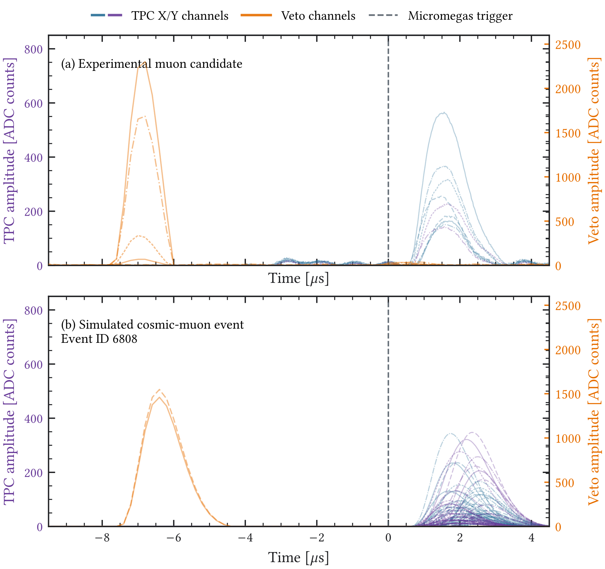
The background model therefore operates on reconstructed observables rather than on ideal deposited energy. The source response depends on whether an interaction survives waveform formation, channel thresholds, hit reconstruction, track building, and the stated analysis contract.
6.2.5 Analysis processes and observables
The common analysis chain is kept in one version-controlled configuration so that simulated and measured events enter the same reconstructed observable space. Simulation-only stages apply the detector-response model before digitization, whereas measured data enter as acquired waveforms. After this input-specific boundary, both follow the same baseline correction, peak finding, hit reconstruction, and topology analysis. Truth observables remain available for validation and mechanism studies but are excluded from the experimental selection.
The response model contains the effects that materially alter the low-energy selection. Lindhard-type ionization quenching is applied to identified gas nuclear recoils, while Birks saturation is applied to highly ionizing deposits in the scintillator [109, 110, 113]. In a representative cosmic-neutron validation sample, the energy-weighted visible energy in the gas changes by only about 0.22% on average because only a small subset of deposits is recoil-like. The corresponding scintillator visible signal is reduced by about 25.7%, so veto thresholds are appreciably sensitive to the Birks and light-collection assumptions. Photon deposits, including capture-gamma deposits, are left unquenched.
Scintillator light is attenuated according to the distance to the effective readout end, and the same path supplies a propagation-time correction. This effective model captures the leading position dependence of the long veto panels without an optical-photon simulation; reflections, surface treatment, coupling, and channel gain are absorbed into calibrated parameters.
TPC ionization is broadened using gas-dependent transverse and longitudinal diffusion coefficients obtained from Garfield++/Magboltz. An empirical hit-smearing stage accounts separately for residual energy-resolution effects not described by diffusion alone, including gain, avalanche, electronics, and calibration broadening. The exact equations, nominal constants, validation sample, and implementation inventory are retained in Appendix Section A.1.2.
Waveform formation uses separate sampling, shaping, trigger, and calibration settings for the TPC and veto branches. The Micromegas scale is anchored to the reconstructed peak, while the veto scale is aligned to the measured through-going-muon response panel by panel. The resulting time-structured waveforms are processed with the same channel masks, noise corrections, peak definitions, and readout mapping used for data rather than treated as deposited-energy sums.
The final TRestAnalysisTree observables include reconstructed energy, valid-track counts, fiducial position, hit and width summaries, projection balance, and veto timing and multiplicity. These reconstructed quantities, not source identity or transport truth, define the selections and source-response factors used below.
6.2.6 Reference samples for selection and normalization
In addition to source-specific background simulations, dedicated reference samples were used to characterize the response to X-ray-like events and to validate the selection criteria. These samples are not background components: their purpose is to define the signal acceptance of the reconstruction and to provide a controlled reference against which background events can be selected or rejected. They therefore occupy a central position between the detector-response model and the final source-normalized background table.
Two classes of signal-like simulation samples were used for this purpose. The first class consists of -like calibration simulations. The dominant manganese line at lies inside the axion-search energy interval and produces compact photoelectric conversions in the gas. This sample is used to validate the response near the standard calibration energy and to compare the simulated reconstructed spectrum with measured calibration data, as discussed in Section 3.6.1. The same sample also exposes fluorescence-induced, multi-site topologies that fail the one-track requirement. A representative reconstruction is retained with the supplementary selection diagnostics in Figure A.5.
The second class consists of uniform low-energy X-ray simulations, in which primary photons are generated over a flat 0–12 keV energy range. This sample maps the selection efficiency across the full low-energy region rather than only at the line. The full sample-role and configuration map is given in the appendix. In summary, source-specific simulations provide the rejection diagnostics, while measured calibration data provide the accidental-veto model.
The production campaign keeps the calibration and background samples gas-matched. For the candidate-v1 study summarized below and the cosmic diagnostics retained in Appendix Section A.9, the , muon, and neutron samples were reconstructed with the same argon–isobutane detector-response settings used by the IAXO-D1 simulation chain. Equivalent -- calibration productions are also part of the broader BabyIAXO program, but they are combined only with background samples reconstructed with the same gas, pressure, drift field, and readout configuration. Keeping the reconstruction stage identical is essential: the efficiencies must be expressed in terms of the same observables that are later applied to the background components. In practice, the most relevant reconstructed quantities are the fiducial or readout-plane energy, the number of reconstructed hits, the spread of the charge cloud in the readout plane, the balance between the two strip directions, and the track observables produced after hit clustering.
The deterministic Micromegas reference selection is
(6.1)
where selects the reconstructed energy region of interest, requires one valid maximum track in each strip projection, and requires the maximum-track center to lie within of the readout center. The stages are applied in that order: energy, one-track reconstruction in both projections, and the fiducial criterion. Learned topology selections are evaluated only as diagnostics and are not factors in . The full signal efficiency must be defined in bins of true incident photon energy,
(6.2)
The denominator must include generated photons that fail to interact, reconstruct, or enter the analysis tree. The distinction between this complete-denominator efficiency and the conditional topology response of the legacy retained-event sample is formalized with the detailed response tables in Appendix Section A.1. The sample provides a complementary check at the calibration energy: it tests whether the Monte Carlo response produces the same compact event population, reconstructed peak position, and peak width observed in measured calibration data.
6.2.6.1 Machine-learning study of an X-ray-like topology cut
The topology study tested whether reconstructed Micromegas shape information could add rejection after the deterministic energy, one-track, and fiducial requirements. Its principal candidate, background-analysis-v1, is a boosted decision tree trained on gas-matched simulated and cosmic-background samples using only reconstructed charge-width, hit-multiplicity, skewness, energy-sharing, and projection-balance observables. Reconstructed energy, source identity, particle type, transport history, and other simulation-only information are excluded from the feature vector. The working point was frozen at 80% acceptance of an untouched simulated partition before comparison with measured calibration data.
The BDT was compared with binned log-odds, sequential interval cuts, and lower-capacity models. These comparisons established that topological information is present in the reconstructed variables, but they do not establish a transferable rejection factor. The exact feature vector, score definitions, smoothing choices, thresholds, random seeds, grouped evaluation, and complete method survey are documented in Appendix Section A.1. The main chapter retains the two tests that determine whether any learned rejection may enter the background model: simulation-to-data transfer of the frozen candidate and independent run-disjoint validation of a bounded repair family.
The complete method-development comparison is given in Table A.4. It motivated the multivariate study but is not an independent production-rate evaluation and supplies no rejection credit to the conservative reference.
The complete run-block closure and candidate-v1 gate audits are given in Table A.5 and Table A.6, respectively. The decisive results are summarized here. On the untouched August–September block, the calibration-anchored BDT retained of calibration events but also accepted of background candidates. For the transfer test, the same simulation-trained model and its frozen threshold are applied to measured R02756 without retraining. It retains of untouched simulated events but only of the measured calibration, so it fails detector-domain transfer. The same model accepts of the simulated production-holdout cosmic candidates. This cosmic value and the wider group-safe cross-fit result are diagnostics, not experimentally validated background acceptances.
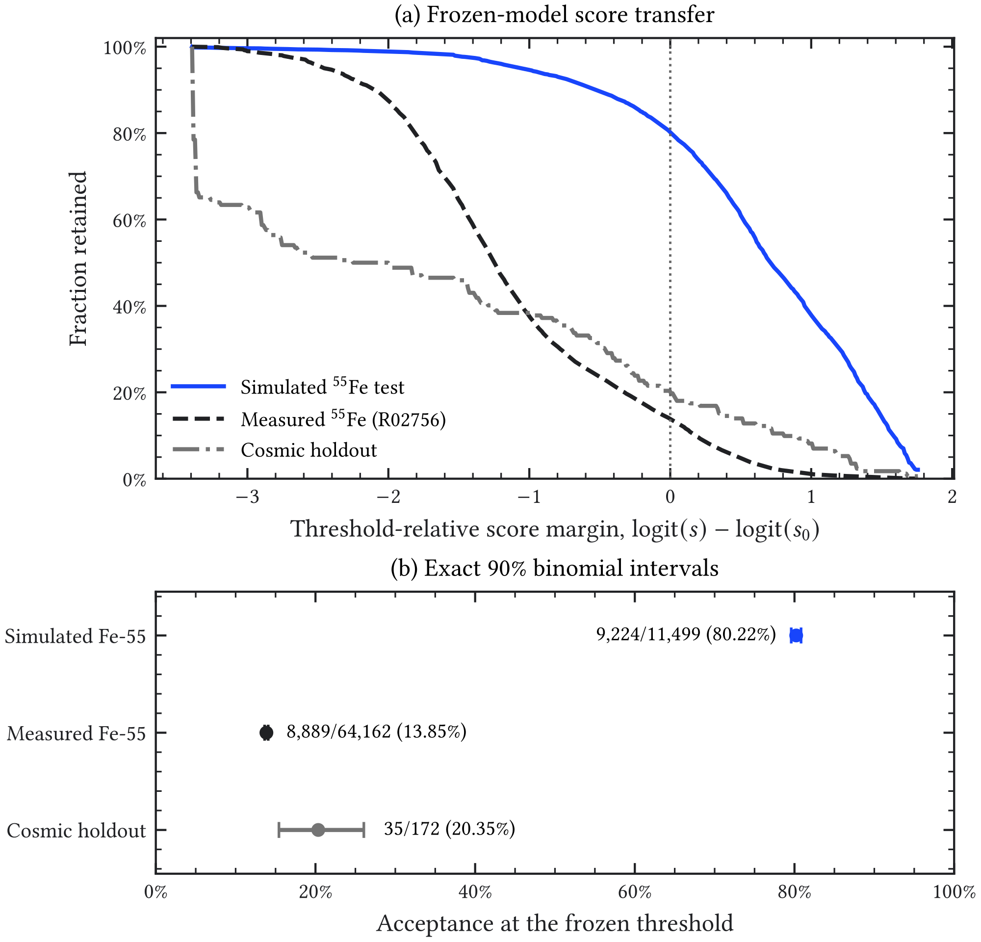
Figure 6.3 contains the decisive promotion test. The classifier orders the untouched simulated X rays above many simulated production-holdout cosmic candidates, but the measured population moves predominantly below the same frozen boundary. The failure is therefore one of detector-domain transfer, not merely a choice of operating threshold. The supporting observable ECDFs, grouped importance/domain-shift comparison, and physically consistent response slices are retained in Figure A.6, Figure A.7, and Figure A.8, respectively.
A post-failure ablation study found no feature subset or lower-capacity model that met the joint signal-transfer and group-safe cosmic-rejection screen. Because this study was designed after observing R02756, it remains development evidence and cannot validate a successor selector. Its exact gates, candidate definitions, and outcomes are retained in Appendix Section A.1.
A final bounded repair family was then predeclared on independent 2025 IAXO-D1 argon runs before the reserved R03018/R03015 blind block was opened. Exactly three candidates were allowed: a calibration-anchored logistic model, a robust signal-distance score, and a transparent five-feature interval box. Their thresholds were fixed on R02997 and evaluated on the independent R02998 calibration and R02993/R02994 background samples. Table 6.4 gives the resulting promotion test; the detailed run-quality and exclusion record is provided in the appendix.
| Predeclared candidate | Independent non-blind validation | Promotion result |
|---|---|---|
| Calibration-anchored logistic, 15 features | Signal (R02998): , 90% C.I. –. Background (R02993+R02994): , 90% C.I. –. | Signal gate passed; background upper bound exceeded the predeclared 25% limit. |
| Signal-only robust L1, 15 features | Signal (R02998): , 90% C.I. –. Background (R02993+R02994): , 90% C.I. –. | Failed the 75% signal lower-bound gate and the background gate. |
| Transparent five-feature box | Signal (R02998): , 90% C.I. –. Background (R02993+R02994): , 90% C.I. –. | Failed the signal point, signal lower-bound, run-range, and background gates. |
The decision was deterministic: the result records selected_candidate=null and blind_input_opened=false. The R03018/R03015 block therefore remains unopened for selector evaluation, and the failed non-blind result was not followed by retuning. The logistic candidate reproduced the nominal signal working point, but failed promotion decisively: its background acceptance demonstrates that the tested feature representation does not provide transferable rejection under the independent run conditions. Consequently, the conservative thesis reference assigns no learned topology-rejection credit.
The frozen candidate-v1 response was also evaluated versus energy with a uniform-X-ray argon production. Its conditional and incident-chain topology efficiencies are retained in the appendix because the selector fails the measured-signal domain gate and therefore cannot define the thesis signal efficiency. The companion saveAllEvents production is nevertheless important: it retains every generated photon, including non-interactions and reconstruction failures, and supplies the complete incident denominator needed for the reference-selection reference.
The same complete ledger also permits the reference-selection efficiency required by the conservative reference to be evaluated without a new transport campaign. Table 6.5 stops the cut flow after the energy, one-track, and fiducial requirements. It is therefore independent of both failed topology studies.
| True incident energy [keV] | Generated | Pass conservative reference | Incident-reference efficiency [%] |
|---|---|---|---|
| 2.0–2.5 | 41885 | 7333 | |
| 2.5–3.0 | 41726 | 8815 | |
| 3.0–3.5 | 41801 | 10519 | |
| 3.5–4.0 | 41561 | 12113 | |
| 4.0–4.5 | 41497 | 12401 | |
| 4.5–5.0 | 41531 | 12463 | |
| 5.0–5.5 | 41912 | 12241 | |
| 5.5–6.0 | 41754 | 10920 | |
| 6.0–6.5 | 41712 | 9001 | |
| 6.5–7.0 | 41712 | 6338 |
The conservative incident-reference efficiency peaks at in the – bin. Integrated over the flat generated spectrum in the – true-energy interval, of the incident photons pass the conservative reference, with a 90% confidence interval of –. This is the thesis reference response for the specified calibration-like illumination, rather than a final axion efficiency. An optics-weighted BabyIAXO efficiency must additionally use the Xe–Ne detector response, the telescope point-spread function and spectrum, and separately measured veto/live-time losses.
The two independent validation routes lead to the same conclusion. Candidate-v1 fails simulation-to-data transfer, and the bounded 2025 family fails the non-blind background gate despite recovering the nominal calibration working point for one candidate. Shared reconstructed branch names do not establish detector-domain closure, and no learned topology-rejection factor is credited in the conservative reference. The feature-level domain diagnostics, historical selector comparisons, run-block studies, and candidate-v1 response tables remain in Appendix Section A.1. Any future learned selector will require new run-group-independent evidence; it is not a prerequisite for the deterministic thesis reference.
The veto stage follows three accounting rules established in Section 5. For an uncorrelated X-ray signal, veto loss is accidental and the survival probability is
(6.3)
where must be measured from an appropriate noise overlay or data control. For prompt-correlated backgrounds, a validated reconstructed veto selection may be credited separately. For delayed activation, the initiating shower is outside the Micromegas-trigger coincidence window and no prompt-veto rejection is credited. The uniform-X-ray production does not yet include an accidental overlay, and the current source frames do not match the calibration-noise domain of the design classifier; both therefore remain pre-veto in the conservative reference.
The final source contribution is obtained by combining the raw source normalization with the event-level survival of the X-ray-like selection and the source-appropriate veto treatment. For a source , the most general expression is a weighted sum over reconstructed events,
(6.4)
where contains the source normalization and any geometrical, spectral, live-time, activity, surface, or phase-space weight assigned to event , and equals one when the event satisfies . The source-specific selection includes and, when applicable, the reconstructed-veto survival criterion. For delayed-activation components, it includes no correlated prompt-veto rejection. A separately measured accidental-veto or live-time survival factor may still apply to the delayed channel. For an unweighted prompt sample generated directly from the physical source distribution, Equation (6.4) reduces to ; the delayed case uses with respect to the correlated prompt veto. Depending on the source component, the raw normalization is derived from a material activity, a measured environmental flux, a cosmic-ray flux model, or an experimental live-time normalization.
For one fully specified and mutually exclusive source hypothesis , the total predicted background rate in the region of interest is then
(6.5)
with analogous sums before cuts and after X-ray-like cuts alone. Alternative gas scenarios and alternative descriptions of the same neutron field are never included together in . Likewise, an aggregate HENSA row cannot coexist with its prompt and delayed subchannels, whereas the two disjoint prompt and delayed subchannels may each appear once. This three-stage presentation is useful because it separates the physics source model from the detector selection:
the raw rate before analysis cuts tests the source normalization and geometry;
the rate after the deterministic Micromegas reference tests whether the component produces a valid low-energy, one-track event in the central fiducial region;
the rate after the reference plus a source-appropriate veto tests the residual background after the active-shielding strategy is applied, without assigning prompt-veto rejection to delayed activation.
The background tables are organized, for each source component, around the number of simulated events, the number of analyzed events, the X-ray-like selection efficiency, the veto survival fraction, the raw normalized level, and the residual level after all selection stages. This structure allows transport samples to be reused when only reconstruction or selection changes. The source tables presently include candidate-v1 results and earlier snapshots such as fe55-shape1014-ld165-td063-bin234-v1. The latter detector-response nickname does not identify a unique event selector: the audit found transparent interval cuts, legacy BDTs, energy-binned cuts, and both and fiducial objects under related labels. Each table therefore states its actual analysis treatment. Only rows explicitly marked as compatible with background-analysis-v2-conservative-reference enter the thesis partial reference; candidate-v1 and legacy rows remain diagnostic or await reprocessing.
Monte Carlo statistical uncertainties use 90% counting intervals [114, 115]. Ordinary equal-weight counts receive central Garwood intervals. Rows with zero, one, or two survivors are reported as one-sided upper bounds corresponding to , , or equivalent Poisson events, respectively; each bound is propagated through the same source and area normalization. Unequal-weight strata are treated separately before combination, and legacy rows without the required bookkeeping remain auxiliary. The complete interval convention is documented in Appendix Section A.1.3.
6.3 Measurement inputs and normalization strategy
The measurements used in this chapter do not constitute a single background data set. They enter the model in three distinct ways. Material-screening measurements provide activity normalizations for intrinsic radioactivity. Environmental and cosmic-field measurements define source terms for particles entering the detector from outside. Detector background data provide validation samples and operational constraints for the reconstruction, veto response, radon handling, and residual event interpretation. This separation is important because a measured activity, a measured external flux, and a measured detector rate constrain different parts of the calculation.
6.3.1 Material screening and radiopurity inputs
Radiopurity screening provides the activity normalization for the intrinsic-background part of the model. The measurements summarized here are collaboration inputs, principally from the Zaragoza detector and radiopurity teams and from work performed at the Canfranc Underground Laboratory (LSC); they are not claimed here as an original contribution of this thesis. They are nevertheless essential to the simulation chain, because every activity limit or measured contamination level must ultimately be translated into an expected event rate in the Micromegas region of interest.
The screening strategy follows the low-background Micromegas program developed for CAST, TREX-DM, and the IAXO prototypes [16, 116, 117]. Material samples are measured mainly with ultra-low-background high-purity germanium (HPGe) detectors at LSC, where the underground overburden suppresses the cosmic-ray component of the counting background. The relevant gamma-emitting isotopes and decay-chain segments include , , the chain, and the / chains. For the background model, the outcome of these measurements is a set of specific activities, or upper limits, assigned to detector volumes such as the Micromegas readout, field cage, cathode, chamber, shielding, calibration hardware, cables, and electronics. Upper limits are retained explicitly because many selected materials are sufficiently clean that no statistically significant peak is observed in the screening spectrum.
The IAXO-D1 screening compilation draws principally on the TREX-DM and Micromegas material-screening campaigns [78]. Most material activities in the present model are upper limits and must therefore be interpreted as conservative bounds on their background contributions rather than as measured central values. The activity assumptions for in the gas, in the lead shielding, and in the readout are identified separately in the source-specific tables.
The radiopure-electronics program is another collaboration input that affects the material inventory close to the detector. E. Picatoste reported the status of the Micromegas radiopure electronics at the 21st IAXO Collaboration Meeting, including the production and testing of front-end flex circuits, limandes, and FEC/BEC interconnect elements intended to reduce the amount of non-radiopure material inside the shielded volume [76]. This work is relevant for the background model because the electronics are geometrically close to the gas volume and can therefore contribute through compact low-energy deposits or through secondary radiation produced in nearby materials. For this reason, the final detector model must distinguish between material located inside the radiopure boundary and services or back-end electronics that are farther away or shielded differently.
| Input source | Detector elements | Use in the background model |
|---|---|---|
| Published Micromegas radiopurity program | Microbulk readouts, vessel materials, field cage, calibration components, shielding samples | Establishes the baseline material-screening methodology and provides activity measurements or limits for materials already used in CAST, TREX-DM, and IAXO-related Micromegas detectors [16, 116, 117]. |
| LSC and Zaragoza IAXO-D1 screening inputs | Readout, aluminized PET and cathode materials, lead shielding, copper and structural elements | Provides the activity normalization for the intrinsic-radioactivity simulations in the IAXO-D1 model; most entries are upper limits, while the assumptions for , , and readout are stated separately in the corresponding source-specific [78]. |
| Radiopure-electronics development | Front-end flex circuits, limandes, FEC/BEC connection elements, nearby service materials | Defines which electronics components can be placed near the detector and which volumes should be represented explicitly as possible internal-contamination sources [76]. |
| IAXO-D1 operation at LSC | Shielded detector, gas system, radon-suppression configuration, calibration hardware | Provides validation data and operational constraints for the model, especially for separating intrinsic radioactivity from gas-borne radon, surface contamination, and residual environmental backgrounds [78, 118, 119]. |
Radiopurity measurements alone do not determine the low-energy background, because the detector response depends on where the isotope is located, on the geometry between the source and the gas volume, and on the subsequent reconstruction cuts. The procedure used in the model is therefore to simulate each relevant isotope–volume pair with Geant4, process the surviving events with the same analysis chain used for experimental data, and only then scale the accepted rate by the measured activity or upper limit. The corresponding intrinsic-contamination simulations are described in Section 6.4 as part of the full production inventory.
6.3.2 Environmental and cosmic source measurements
External source terms are constrained by measurements and generators in a different way from material screening. For surface cosmic-ray backgrounds, CRY, analytic muon parameterizations, EXPACS, and HENSA measurements define the incident particle spectra used in the detector simulations. For laboratory environmental radiation, NaI and HENSA measurements provide local gamma and neutron fields that can be propagated through the detector geometry. These inputs are source terms, not detector backgrounds by themselves: they become a predicted Micromegas rate only after transport, detector response, reconstruction, and the X-ray-like selection.
The Zaragoza laboratory measurements and HENSA-based neutron spectra are therefore used as source-term anchors for the simulations discussed in Section 6.5. They are especially useful for testing the response of the shielding and veto system to realistic neutron fields. However, the corresponding absolute rates remain site dependent. A future DESY-specific characterization of the gamma field, ground and nearby materials, local structures, and neutron environment is needed before the same source inventory can be converted into a BabyIAXO site prediction.
6.3.3 Detector background data and operational constraints
Detector data are used primarily to validate the reconstruction and to constrain operational background mechanisms. The surface-veto validation uses the published IAXO-D0 prototype data set [17]; the HENSA-driven simulations are used to study the neutron response of the selected three-layer design-study geometry; and environmental gamma or material-produced neutron studies are retained as source-specific checks until their DESY normalization is fixed. This separation avoids mixing measured detector performance, simulated source transport, and site-dependent absolute fluxes into a single number without stating the assumptions behind it. The historical response scale in Appendix Section A.6 is therefore built from explicit scenario choices and upper bounds rather than from an implicit combined fit to detector data.
The LSC IAXO-D1 data sets also show why the material model must be complemented by operational background studies. The detector was operated inside a 20 cm lead shield with a calibration source, nitrogen or radon-free-air flushing inside the shielding, and evolving gas recirculation and buffer configurations [78, 118, 119]. Those measurements showed that changes in gas handling and radon suppression can affect the alpha and low-energy backgrounds substantially, even when the solid materials have been selected for radiopurity. Consequently, the background model separates intrinsic material radioactivity from radon-related and surface-contamination components, rather than absorbing all observed low-energy events into a single material-activity term.
6.4 Intrinsic background
6.4.1 Gas-borne and radon-related contamination
The IAXO Micromegas detector is designed to operate with either an argon-based gas mixture or a xenon–neon-based gas mixture. Because the active gas is the interaction medium, its isotopic composition and any gas-borne radioactive contaminants must be treated separately from the solid detector materials. Common gas impurities such as oxygen and water affect electron attachment, gain stability, and energy calibration, but their concentrations and natural isotopic composition do not make them relevant radioactive-background sources. The radiological gas model is therefore dominated by two classes: intrinsic radioisotopes in the gas itself and radon-related activity introduced by emanation, leaks, or recirculation.
For argon mixtures, the relevant intrinsic isotope is , a beta emitter with and . Natural atmospheric argon has a measured specific activity of of natural argon [120]. The absolute rate therefore scales with the gas inventory and with the choice of atmospheric or underground argon; low-radioactivity underground argon has been measured to suppress by a factor relative to atmospheric argon [121]. beta decays generally produce extended ionization tracks rather than compact few-keV X-ray-like clusters, and legacy selectors consequently predict strong rejection. The conservative reference nevertheless credits no learned topology-rejection factor until this source is rescored with a detector-domain-validated selection.
provides a second gas-borne beta-decay scenario for argon-based operation when krypton traces remain in gas distilled from air. Its half-life is , with , and its activity can vary strongly between gas batches and handling histories. The GERDA collaboration measured a specific activity of in an atmospheric liquid-argon batch, while also noting the broader atmospheric and experiment-dependent variability of this isotope [122]. The simulation is therefore treated as a scenario component normalized by an assumed gas activity, not as a fixed property of the detector materials.
Radon must be handled differently from ordinary material-chain activity. As a noble gas, can escape from surrounding materials or gas-system components and break secular equilibrium with the parent uranium chain. Its concentration in the detector volume is consequently an operational quantity, set by emanation, leaks, flushing, recirculation, and gas purification rather than by the bulk activity of a single detector material. The most relevant isotope for this model is , with . It acts first as a uniform gas source, but its daughters can become surface sources after ion drift or plate-out.
The separation between the radon components is important because each component has a different normalization. , the first short-lived daughter of , is often positively charged after production and can drift toward the cathode under the detector field. Long-lived , with , can then remain on detector surfaces and is not generally in equilibrium with the instantaneous radon activity. For this reason, and following the surface-contamination concern motivating dedicated screening with Micromegas detectors [123], the model treats gas , cathode , cathode , and vessel or surface as separate source hypotheses. The source taxonomy is summarized in Table 6.7.
| Source | Model location | Normalization input | Background-model role |
|---|---|---|---|
| Uniform active gas, only for argon mixtures. | Argon mass multiplied by the selected specific activity; atmospheric and underground argon are distinct assumptions. | Beta source with mostly extended ionization; retained as a gas-intrinsic source component with no learned topology rejection credited in the conservative reference. | |
| Uniform active gas, for krypton traces in argon mixtures. | Gas inventory multiplied by an assumed activity; batch history and air-derived contamination dominate the normalization. | Beta source used as a gas-purity scenario and normalized separately from . | |
| Uniform gas activity in the active volume. | Measured or assumed gas activity after emanation, leaks, flushing, and recirculation are specified. | Time-dependent gas-borne source; useful for testing radon-handling scenarios rather than a fixed material-screening term. | |
| Cathode or window surface after ion drift from the gas. | Radon activity combined with an ion-collection or plate-out fraction. | Surface alpha source close to the sensitive gas; treated separately from uniform radon because the geometry and topology change. | |
| Cathode, vessel, or other gas-facing surfaces. | Surface activity or exposure history; not assumed to be in equilibrium with the current radon concentration. | Long-lived beta/gamma surface component that can persist after the gas radon level changes. |
The gas and radon simulations resolve the detector response for distinct source locations. They use the fe55-shape1014-ld165-td063-bin234-v1 argon–isobutane reconstruction, including the maximum-track energy and fiducial definition. Table 6.8 retains the source-filtered and reconstructed counts; the last column is an auxiliary transparent-topology diagnostic and receives no rejection credit.
| Source | Stored | Processed | 2–7 keV | Fiducial | Legacy topology |
|---|---|---|---|---|---|
| gas | 100000 | 62051 | 13164 | 357 | 28 |
| gas | 100000 | 62160 | 13861 | 377 | 29 |
| gas | 100000 | 59856 | 357 | 15 | 0 |
| cathode | 100187 | 99950 | 5500 | 697 | 14 |
| cathode | 100145 | 99901 | 10990 | 3009 | 68 |
| vessel | 99723 | 98482 | 3916 | 0 | 0 |
For source activity , the physical response is
Here counts generated parent decays before event filtering, with the simulated chain segment specified. The preserved count table does not establish that denominator. The earlier conversion using stored entries is therefore not retained as a per-becquerel result; subsequent analyses require an explicit generated-parent ledger, and chain subevents retain their common parent identity for uncertainty estimation.
The activity inputs can nevertheless be stated independently of detector acceptance. The active volume at , , and argon corresponds to approximately of argon. Table 6.9 separates the literature benchmarks from operational radon and surface-contamination hypotheses.
| Source scenario | Activity input | Physical interpretation |
|---|---|---|
| Atmospheric | of Ar | Measured atmospheric benchmark; multiply by the argon mass. |
| Underground-argon | Atmospheric benchmark divided by | Alternative gas choice; procurement and batch history remain relevant. |
| in argon | of Ar | Reference value from one measured atmospheric-argon batch. |
| Gas | Illustrative clean-gas concentration, set by emanation, flushing, and recirculation. | |
| Cathode / | for each source | Independent surface hypotheses; collection efficiency and exposure history determine the actual activities. |
Surface contamination requires an implantation-depth or plate-out distribution as well as an activity. Short-lived daughters need not remain at the original gas-decay position, and long-lived is not in equilibrium with the instantaneous radon concentration. Existing alpha and gas-handling controls can constrain these source classes without fitting each activity independently to the sparse X-ray background data. Representative ionization topologies are shown in Appendix Section A.3.
6.4.2 Detector materials
The detector materials are selected and screened with particular attention to components close to the active gas volume, where low-energy photons or charged particles can reach the Micromegas readout with little additional attenuation. For the background model, the most relevant material classes are:
Copper: the main chamber and local shielding material, also present near the readout plane and in some electronics structures.
Lead: the passive shielding material. General-purpose lead can contain substantially larger activity than the copper chamber, so the detector-facing lead layers are treated explicitly.
Stainless steel: a structural material for supports, platform elements, and beamline connections. It is minimized near the sensitive volume and treated mainly as a geometry- and screening-dependent source.
Kapton: a polymer used in the Micromegas readout plane and flex structures. Its radiopurity is important because it is close to the charge-collection region.
PTFE: an insulating and low-outgassing polymer used in detector components close to the sensitive gas volume.
Aluminized PET: the thin entrance-window/cathode material above the central region where focused axion-induced X-rays are expected to convert.
Front-end electronics materials: mixed PCB and component materials that must be close to the detector for signal integrity, but are difficult to represent with a single homogeneous radiopurity value.
The radiopurity program follows the low-background Micromegas experience from CAST and related detector developments, but the relevant activity vector is still component specific. High-purity germanium measurements at the Canfranc Underground Laboratory provide activities or upper limits for many candidate materials, including auxiliary components such as epoxies and glues. These screening inputs define source scenarios for the material response. A screening upper limit can set a conservative activity scenario, but its product with a simulated acceptance is not automatically a confidence bound on the total background. Uranium- and thorium-chain segments must be normalized independently unless secular equilibrium is demonstrated; an early-chain assay does not determine the late-chain or surface activity. For the copper and lead components, auxiliary standalone decay-transport simulations were also produced to verify the source construction before running the full detector-level background simulations. These diagnostics score photons and electrons as they escape the material volume, retaining their energy, exit angle, and parent depth. Each material/isotope configuration contains generated decays, split into independently seeded simulation shards; the uncertainty bands in the figures are the corresponding Poisson statistical uncertainties after combining the shards. The plots are therefore used as transport and source-depth checks, not as standalone background-level estimates.
6.4.2.1 Copper parts
Electroformed copper has very high chemical purity, but the relevant background source is its residual radioactive content and activation history rather than its elemental purity alone. The copper source inventory includes , , , and . Among these, is especially important because it can be produced by cosmic-ray activation. Its activity depends on the exposure history of the copper, and a surface experiment does not benefit from the long underground cooling periods available in some low-background facilities. The dedicated HENSA inventory in Section 6.7 observes 124 products in simulated neutrons. The same study finds more frequent production of shorter-lived copper isotopes; detector coupling determines their relative selected-event yields, while half-lives determine the time dependence.
In the detector-level simulations, copper is treated as a volumetric source of photons and electrons produced by the decay of the isotopes present in the material. The relevant detector-level question is not the MeV-scale spectrum of particles escaping the copper by itself, but the much smaller subset that reaches the gas, deposits energy in the 1–10 keV signal region, and survives the topology selection. The auxiliary decay-transport simulations therefore serve mainly as a consistency check on the source construction: photons can emerge from deeper inside the copper, while escaping electrons are concentrated close to the material surface. This behavior is shown in Figure 6.4, where the photon and electron escape spectra are shown together with the parent-depth distributions.
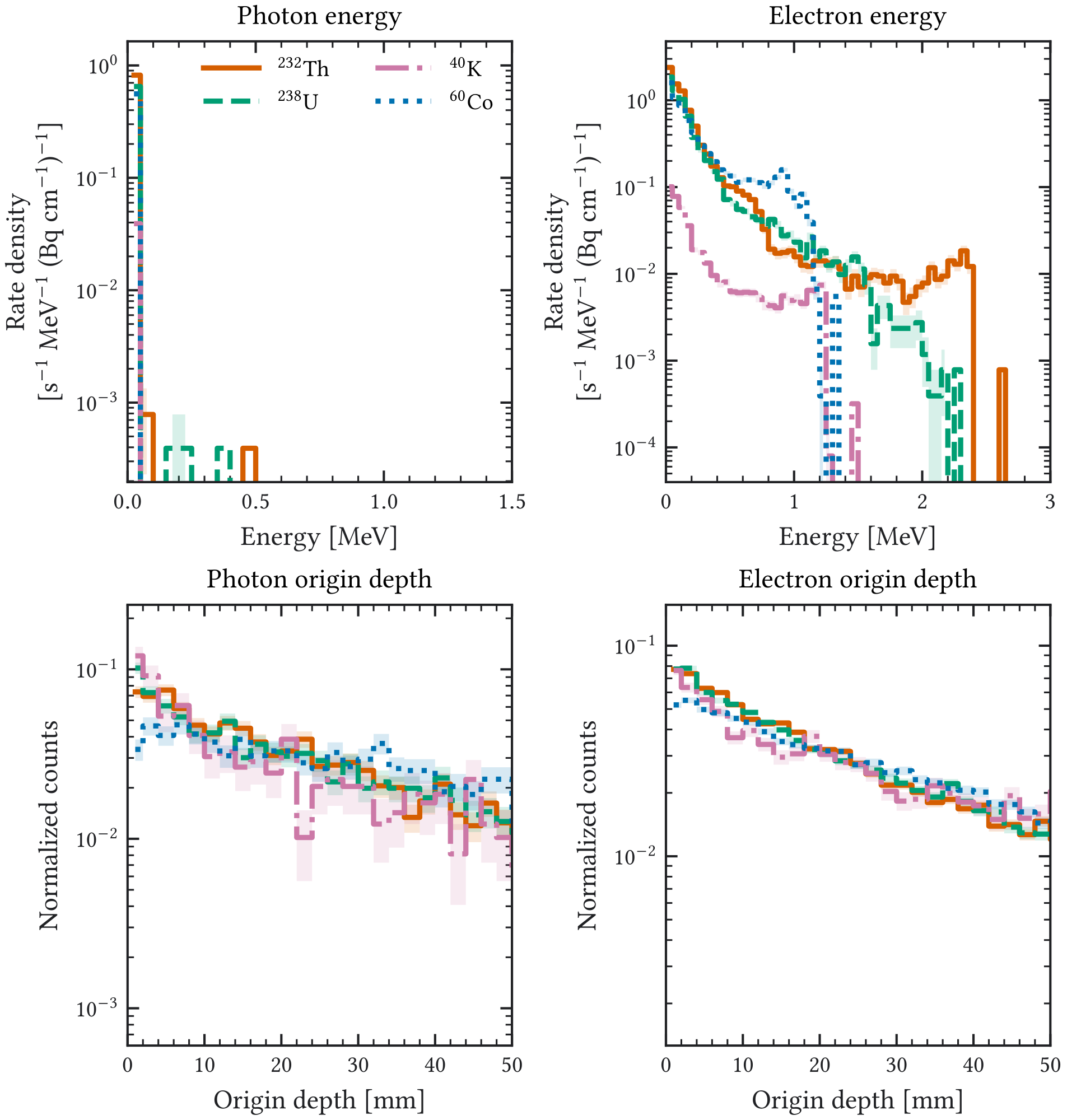
The production threshold and tracking step are distinct numerical controls. A range cut is converted to a material-dependent secondary-production energy threshold; the configured conversion floor does not by itself demonstrate accuracy at the analysis threshold. Likewise, a gas step limit does not replace a production-cut convergence test in copper, lead, the window, or gas. Selected-event yields and low-energy spectral shapes must be compared with tighter region-specific cuts before the material response is assigned a numerical convergence uncertainty.
6.4.3 Telescope and X-ray optics contamination
The telescope-side materials form a separate intrinsic-background source because they are not part of the Micromegas chamber, but they lie on the same optical axis as the focused solar-axion signal. Radioactive decays in the X-ray optics, telescope pipe, or nearby telescope support materials can therefore contribute photons that enter the detector through the magnet-facing aperture rather than through the surrounding shielding. This geometry is qualitatively different from the front-end electronics or shielding sources: most charged secondaries and off-axis photons are absorbed far from the gas volume, while a small fraction of gamma rays emitted into the telescope acceptance can travel along the bore and interact in or near the detector.
The current iaxo-simulations scaffold represents this source with a telescope-side generator volume, telescopePipeGeneratorVolume, and transports the emitted photons through the detector geometry using the standard REST detector-response machinery. It is nevertheless kept separate from the better-constrained intrinsic-background studies because the geometry is an optics-side approximation rather than a screened BabyIAXO optics model, and because the larger production has not yet been reduced with a fully clean, contract-specific analysis output for all files. The first rate-pilot production was generated for the and decay chains. To make the calculation tractable, photons were emitted inside a cone pointing toward the detector. This is an angular-biasing shortcut, not a physical collimation assumption. The pilot rates in Table 6.10 are therefore corrected by the isotropic-cone factor
so that the quoted quantity is the contribution from that cone per becquerel of an isotropic telescope-side activity. The unsampled angular complement is not constrained: scattering in the pipe or shielding can redirect photons initially emitted outside the cone. A full isotropic prediction requires a complementary angular sample or a demonstrated bound on that contribution. A larger production has transported , , and photon source terms, but it has not yet yielded a response-chain-consistent telescope-side result. The telescope-side component therefore remains open until the preserved transport output is reprocessed with a validated response snapshot and the deterministic reference selection.
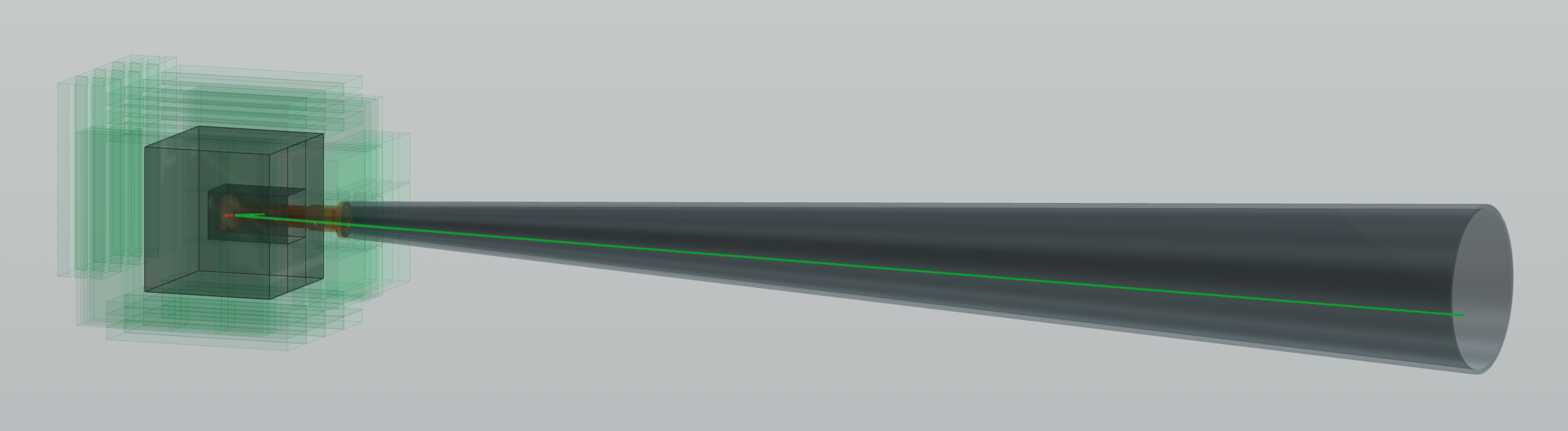
REST-for-Physics event viewer. The long gray volume indicates the telescope-side pipe or optics line, while the detector chamber, shielding, and veto volumes are rendered only as simplified translucent references for readability. The full transport simulation still uses the detector and veto geometry; this view is intended to show the source topology, namely a photon traveling along the optical axis and producing a low-energy detector response near the Micromegas region.| Source | Selection stage | Gamma primaries | Events | Background level per Bq |
|---|---|---|---|---|
| chain | TPC selected | 9 | ||
| chain | Fiducial – | 4 | ||
| chain | TPC selected | 17 | ||
| chain | Fiducial – | 9 |
The pilot establishes a detector-coupled transport path and the normalization of its restricted angular support. The event display in Figure 6.5 confirms that the simulated source can populate the detector through the intended telescope-side path, while the event counts in Table 6.10 guide statistical allocation within the sampled cone; they do not establish the contribution from ungenerated angles. Because the larger production has not yet been reprocessed with a clean, response-chain-consistent analysis output for all files, the telescope-side contribution is not folded into the current source-response budget or the historical response scale in Appendix Section A.6. The final conclusion on the X-ray optics contribution will depend on reprocessing the preserved raw outputs, replacing the generator approximation with the adopted optics-material activity model, and applying the deterministic energy, one-track, and fiducial reference selection. Any source-appropriate veto correction must be validated and reported separately; no BDT or other topology rejection is credited in the present thesis reference.
6.4.4 Front-end electronics
The front-end electronics constitute a special intrinsic-background source because they must be placed close to the Micromegas readout in order to preserve signal quality, while at the same time containing materials that are harder to radiopurify than bulk copper, kapton, or PTFE. This contribution was therefore treated separately from the generic copper and readout-plane contaminations. The simulation described here corresponds to the four front-end cards represented in the IAXO-D1 detector model, without including the flat cables or other service elements. The activity model follows the component-level radiopurity study of the BabyIAXO electronics, used here as a collaboration input rather than as an original measurement of this thesis [76, 124].
The simulated source regions were the four electronics-card bodies located near the Micromegas readout. For each card and each isotope, radioactive decays were generated uniformly inside the corresponding card volume and transported with the same Geant4 physics configuration used for the rest of the intrinsic-background model. The isotopes included in the present production were , , , the chain, the chain, and the chain. The activities assigned to the four cards are summarized in Table 6.11. The optional contribution from the 10 resistors was not included in the nominal normalization because those components were not part of the original low-background board design considered in the reference electronics study.
| Isotope or chain | Four-card activity [Bq] | Per-card activity [Bq] |
|---|---|---|
| chain | ||
| chain | ||
| chain |
The normalization was performed at the level of generated decays. For each isotope–card pair, the event weight was defined as
where is the activity assigned to isotope in card , and is the number of generated decays in that production. This choice is important because only a small fraction of the decays produce a stored detector event, and normalizing to saved or reconstructed entries would bias the rate estimate. The production consisted of 24 isotope–card groups, corresponding to the six isotopes or decay chains in Table 6.11 for each of the four cards. In total, decays were generated and detector events were available for the analysis stage. The chain is the least efficient source in this detector model, and several jobs produced no saved detector event; those jobs were nevertheless retained in the normalization denominator.
The rates are expressed in the background units used throughout this chapter, , using the circular signal fiducial area for the area normalization. This production predates the conservative thesis reference. Its historical post-cut branch applies the energy-binned X-ray topology cuts implemented by the electronics analysis, not the grouped cross-fitted BDT defined above; the BDT wording retained in some generated plot labels is legacy nomenclature. The result is therefore an auxiliary card-response estimate pending conservative-reference rescoring. In this window, before the legacy X-ray cuts are applied, the electronics-card contribution is . The weighted sum of the few post-cut events is , but this is a normalization diagnostic rather than a reported residual level because several constituent rows have at most two survivors.
The post-cut electronics comparison is limited by one or two survivors for several isotope chains. For , one observed event corresponds to the normalization diagnostic , but the reported result is the one-sided bound at 90% confidence. The activity vector and component-level study still identify the ceramic capacitors as an important -bearing source, but the sparse legacy selection does not support a precise ranking of the surviving isotope contributions.
| Isotope or chain | Generated | Saved | Events | – rate | Events | Post-cut rate |
|---|---|---|---|---|---|---|
| chain | 101 | 1 | ||||
| chain | 131 | 2 | ||||
| 105 | 1 | |||||
| 299 | 5 | |||||
| 62 | 2 | |||||
| chain | 4 | 0 |
These results should be interpreted as the card-only electronics contribution for the current detector model and activity vector. They do not yet include flat cables, possible connector materials, or a detailed separation of the individual board components within each card volume. Those refinements are relevant for a future BabyIAXO background model because the activity is not uniformly distributed among components: the activity is concentrated mainly in ceramic capacitors, while resistors, diodes, and chips contribute different isotope mixtures. The card-only production provides a useful first estimate of scale, but its legacy selection and incomplete service-material geometry prevent the result from establishing that front-end electronics are subdominant in the conservative partial inventory.
6.4.5 Shielding
The lead shielding surrounds the detector and is the most massive component in the passive-shielding model. Most electromagnetic emissions from contaminants in the bulk lead are absorbed before reaching the detector. The relevant electromagnetic contribution therefore comes mainly from activity near the detector-facing surface, where photons or electrons can escape the lead and enter the copper and gas region. Neutrons produced in lead by spontaneous fission of or by reactions are treated separately because their penetration length and rejection mechanisms are different from those of charged electromagnetic secondaries.
The shielding model considers , , , , and . Among them, is the most distinctive lead contaminant because its activity depends strongly on the age and handling history of the lead. Its half-life, , is short enough that old or underground-stored lead can have substantially reduced activity. Very low activity lead, including archaeological lead in some experiments, is therefore most valuable in the innermost shielding layers, where it has the largest effect on the detector-facing source term.
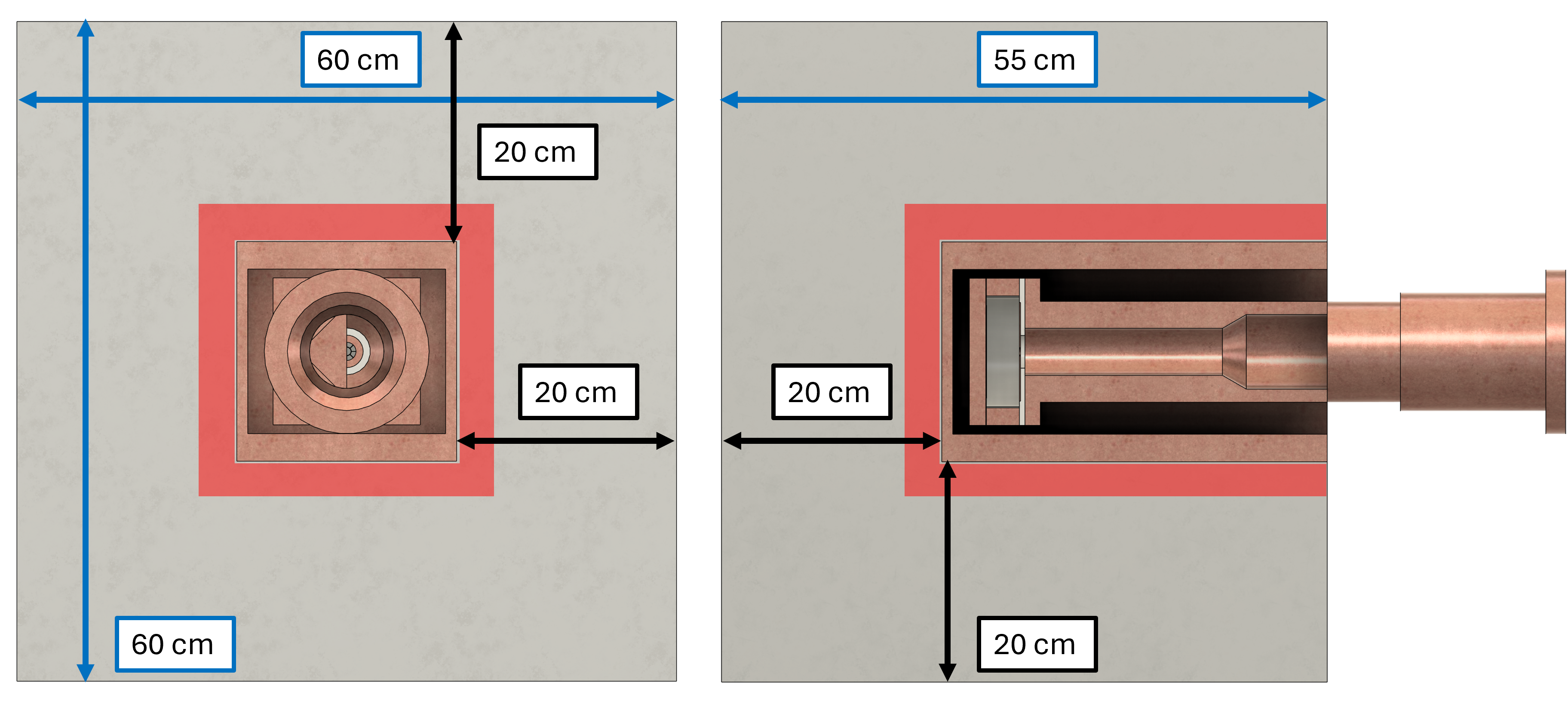
Figure 6.6 shows the segmented shielding geometry used for the detector-level production. The highlighted source region corresponds to the innermost lead layer, a -thick lead shell and the part of the shield most likely to contribute to the Micromegas background. Supplementary escape-particle diagnostics in Appendix Section A.3 show surface-dominated emission, but do not bound the selected-event contribution from deeper lead. The shell is therefore the scope of this result; successive depth shells are needed to demonstrate convergence of a full-lead electromagnetic prediction.
The present production generated decays in this innermost lead layer and normalized them to the activity assumption . Its processed output uses a legacy readout-energy, reconstructed-hit-centroid, and older topology-BDT definition. It is retained as a shielding-response estimate but is not compatible with the maximum-track-centered contract. The completed sample corresponds to 262.5 days of this activity; the production bookkeeping is reported in Appendix Section A.3. After detector response and readout analysis, 1883 events remain in the fiducial – energy window. Only 196 of them have the reconstructed-hit centroid inside the -radius signal region, and two events pass the full TPC/X-ray selection. This geometric check suppresses events that contribute a small reconstructed energy component to the fiducial readout region while the reconstructed charge distribution is actually centered outside the expected axion-window footprint. Because only two events survive, the shielding contribution is quoted as a one-sided 90% confidence upper bound,
The bound uses the one-sided Poisson upper mean for two observed events; it is not the upper endpoint of a central two-sided interval. This snapshot does not assign an independent prompt-veto rejection to , because the current processed files do not contain scintillator-sensitive observables for this source.
| Selection | Events | Fraction of – | Background level |
|---|---|---|---|
| Fiducial – | 1883 | 1.000 | |
| Fiducial – + reconstructed-hit centroid fiducial | 196 | 0.104 | |
| Fiducial – + full TPC/X-ray | 2 | 0.00106 |
The control production in which the detector-facing copper box was replaced by air gives five final TPC/X-ray survivors, corresponding to for the same activity. The higher central response is consistent with attenuation by the copper box, but five control survivors and two nominal survivors do not determine a precise suppression factor.
Additional electromagnetic shielding productions were generated for the activity assumptions , , and . These activities are several orders of magnitude below the adopted activity, and their normalized detector-level contributions after the full TPC/X-ray selection are correspondingly small, as shown in Table 6.14.
| Source | [Bq kg] | Generated decays | 2–7 keV events | Full TPC/X-ray events | Full TPC/X-ray background level |
|---|---|---|---|---|---|
| chain | 79623 | 55 | |||
| chain | 110197 | 108 | |||
| 91312 | 73 | ||||
| 1883 | 2 |
Neutron production in the shield, for example by spontaneous fission or by reactions, is not included in Table 6.14. It is treated as a separate penetrating component because its source volume is the full lead shield rather than only the detector-facing electromagnetic layer, and because the rejection mechanism follows the neutron cascade and veto logic discussed in the external-neutron section. The dedicated full-lead spontaneous-fission neutron campaign has completed its transport and detector-response processing; its detector-level normalization is kept separate from the electromagnetic table while the source term is being defined.
6.5 Environmental background
Environmental components are photons and neutrons produced by the ground, structures, and materials near the detector; atmospheric cosmic-ray secondaries are treated separately in Section 6.6. For BabyIAXO, the current working scenario is an outdoor, on-surface DESY location [15, 67]. The results in this section are detector-response estimates using the available laboratory source terms and are not a final DESY environmental-background budget.
6.5.1 Environmental source model
Environmental radiation refers here to external photons and neutrons produced by the surroundings of the detector, rather than by radioactivity inside the detector materials themselves. This component must be separated from the intrinsic material background discussed above and from the cosmic-ray background discussed later, and it must be carried with an explicit maturity status because its absolute normalization remains site dependent. The first environmental simulations in this work were developed for an enclosed laboratory configuration in which nearby concrete walls, floor, and ceiling were plausible dominant sources of MeV photons and radiogenic neutrons. Those studies remain useful because they established the external-source workflow and the relevant angular distributions, but they are no longer the nominal site model for BabyIAXO. Under the current outdoor, on-surface DESY working scenario, the external field will depend on the ground, local structures, nearby materials, and the cosmic-ray component at the selected location. The results below should therefore be read as detector-response estimates normalized to the best presently available laboratory source terms, not as a final DESY environmental-background budget.
6.5.1.1 Concrete-emission source study
The historical concrete study modeled the natural radioactivity of construction materials through the main gamma-emitting families: K, Th, U, and U. For each isotope, decays were generated uniformly in a -thick concrete slab with effectively infinite transverse size. The auxiliary Geant4 simulation recorded particles that escaped through the surface facing the detector, including their type, kinetic energy, production depth, and exit angle. Only a small fraction of the decay products leave the material, so this two-stage approach avoids repeating the expensive transport through bulk concrete for every detector-response study.
The concrete calculation is not used as the final BabyIAXO source geometry, but it motivated two features that remain in the current detector-level simulations. First, it provides representative MeV-scale photon spectra and event topologies for environmental radioactivity. Second, it shows that the exit-angle distribution of escaping photons is close to the law expected for particles crossing a surface from an approximately isotropic external field, with a small skew toward lower angles due to attenuation at large path length. The detailed concrete spectra and decay-chain diagrams are retained in Appendix Section A.1, while the older detector-level gamma and neutron diagnostics are collected in Appendix Section A.2.
6.5.1.2 External-field generator and normalization
The current detector-level environmental simulations use a compact spherical generator around the closed-pipe detector geometry, as sketched in Figure 6.7. Particles are launched from a sphere of radius , with incidence angles sampled according to . For an isotropic scalar fluence rate , the generated-primary rate is given by the projected area of the enclosing sphere,
(6.6)
The angular projection is already included in this expression, so no additional mean-cosine factor is applied when converting the simulated events into a rate. The resulting events are transported with restG4 and then processed with the same detector-response and X-ray-like selection chain used for the other background components.
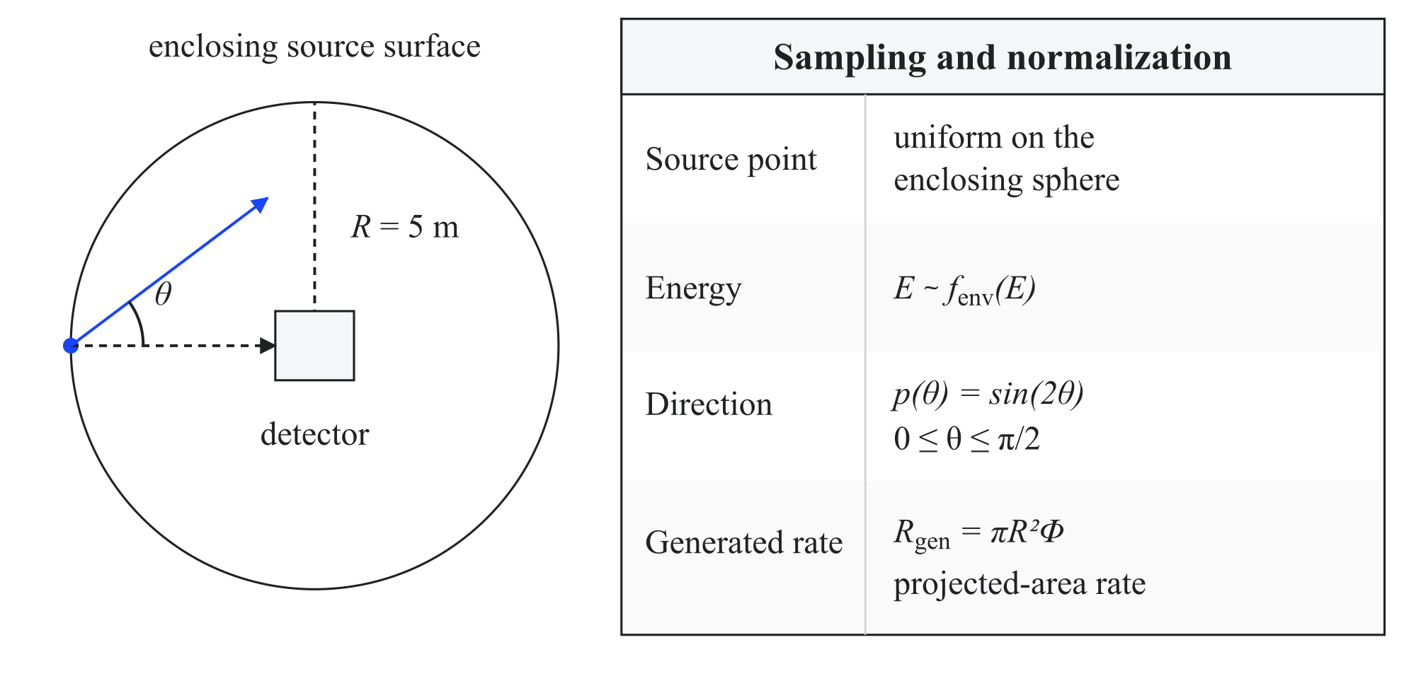
The background level is computed from the number of selected events , the number of generated primaries , the generated-primary rate , the energy-window width , and the signal fiducial area :
(6.7)
This area convention matches the central signal region used for the X-ray-like comparison. If the older full-readout convention of is used instead, the quoted values should be scaled down by a factor .
6.5.1.3 Environmental gammas
The environmental-gamma source represents the non-cosmic MeV photon field produced by natural radioactivity in the surrounding laboratory materials. In the present calculation, photon energies are sampled from the EnvironmentalGammas distribution, , over –. The absolute rate is obtained from the Zaragoza NaI comparison in Figure 6.8. The simulated NaI response is matched to the measured deposited-energy integral between and , , which gives generated photons per measured NaI count. For this fixed spectral template, the resulting generator rate is , equivalent to a fluence of under the adopted -radius source convention. Matching one NaI deposited-energy integral fixes the amplitude of the chosen template; it does not uniquely determine the incident spectrum. Alternative line-plus-continuum spectra can reproduce that integral while producing different low-energy leakage through the shielding. The auxiliary result also excludes incident photons below , above , and the open telescope path. A DESY-specific prediction requires spectral or radiation-map constraints and tests of those omitted regions.
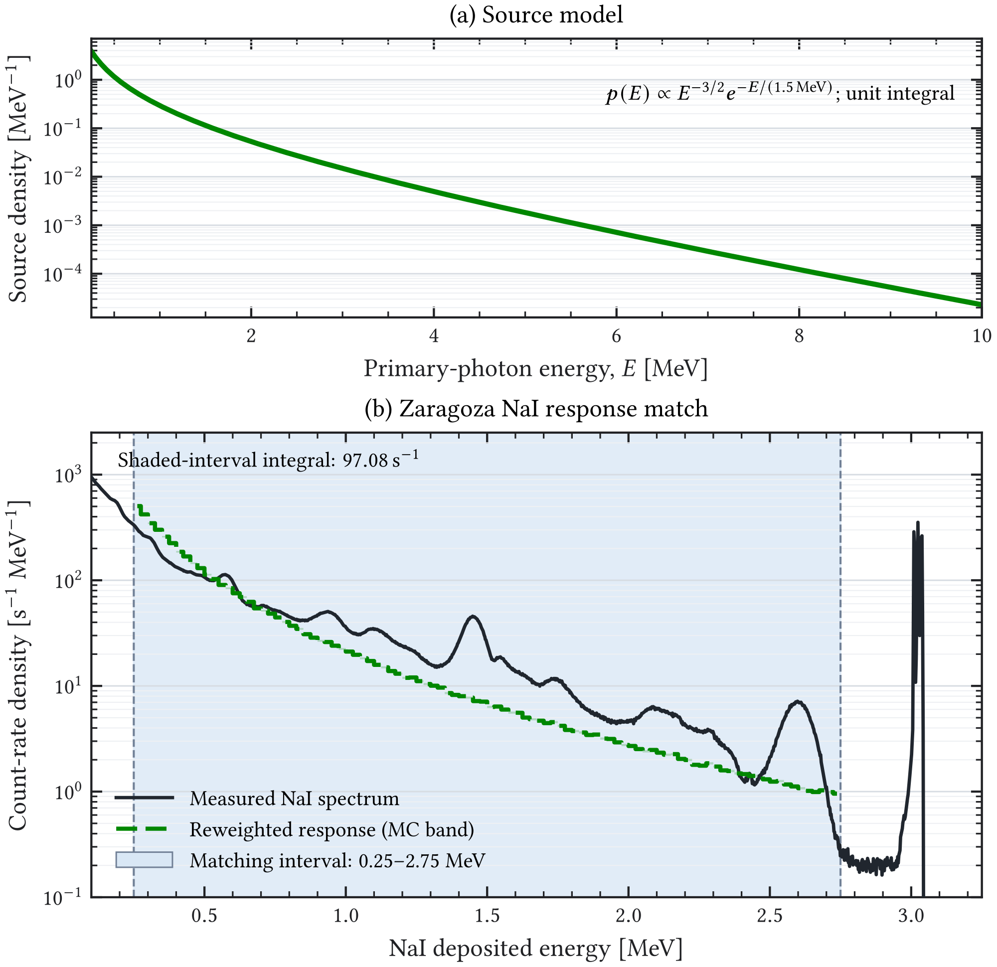
EnvironmentalGammas energy density over its – generator support; the independent incidence-angle distribution is . In the lower panel, the response simulation is reweighted to this source law and scaled so that its integral equals the measured NaI rate of in the shaded – deposited-energy interval; the narrow band around the simulated curve shows its weighted Monte Carlo uncertainty. The narrow measured structure near lies outside that interval, its origin is not assigned in this auxiliary data set, and it has no effect on the normalization.The detector-level production used the closed-pipe geometry with the gas as the only sensitive detector, so that the result estimates the Micromegas background rather than the veto noise response. The campaign generated photons and stored 83 gas-sensitive events. The 79 non-empty transport files were then post-processed with the standard detector-analysis chain. After the X-ray-like cuts, no event remains in the – reference window, so the quoted environmental-gamma contribution is a finite-statistics upper bound.
6.5.1.4 Environmental neutrons
The environmental-neutron treatment evolved during the background-model development. The first diagnostic simulations used a literature-based radiogenic-neutron spectrum for concrete, approximated by an evaporation-like distribution centered around the MeV scale [125]. Those simulations are still useful for illustrating how MeV neutrons can produce low-energy Micromegas deposits through capture gammas and secondary electromagnetic particles, but they are not used as the current normalization. The relevant physical sources of ambient neutrons are instead grouped as follows. First, radiogenic neutrons are produced by reactions in light elements and by spontaneous fission of uranium-series contaminants in concrete, soil, and shielding materials; these processes populate the fast component at the MeV scale. Second, the same radiogenic neutrons, together with cosmic-ray neutrons that scatter in the hall, floor, shielding, and nearby structures, can moderate down to epithermal and thermal energies. This moderated population produces the low-energy peak in the HENSA-derived environmental spectrum, near , while the fast radiogenic and room-return component gives the broader structure around . Third, any remaining site-specific albedo or structure-scattered neutron field is absorbed into the measured HENSA residual rather than assigned to a separate analytic source.
For the present estimate, the neutron source term is the positive HENSA-minus-CRY residual below . Figure 6.9 shows the Zaragoza indoor and outdoor residuals used for the detector-level production, together with one representative DESY indoor and outdoor HENSA spectrum based on the BERT unfolding. The full subtraction diagnostic, including the measured HENSA spectra, the normalized CRY component, and the signed residuals, is provided in Appendix Section A.2, Figure A.10. This residual is a model-dependent decomposition of the measured scalar fluence, not a separately measured radiogenic field. Unfolding, cosmic-model, moderation, and angular uncertainties all enter the subtraction; replacing negative bins by zero biases a noisy residual upward. Correlated unfolded bins must therefore be propagated before the difference is used as a quantitative site comparison. The corresponding Zaragoza integrated fluxes are for the indoor spectrum and for the outdoor spectrum; the DESY BERT indoor and outdoor residuals give and , respectively. The Zaragoza residuals are propagated with the same spherical-source normalization of Equation (6.6) and the same incidence law used for the environmental-gamma production. This construction overlaps the full outdoor HENSA field used later as the nominal cosmic-neutron source. The two must not be added: an additive site model must choose either the full HENSA field or a matched decomposition into a CRY cosmic component plus the HENSA-minus-CRY residual. The environmental residual is therefore retained here as a diagnostic site-transfer decomposition rather than as an additional neutron term beside the full HENSA source.
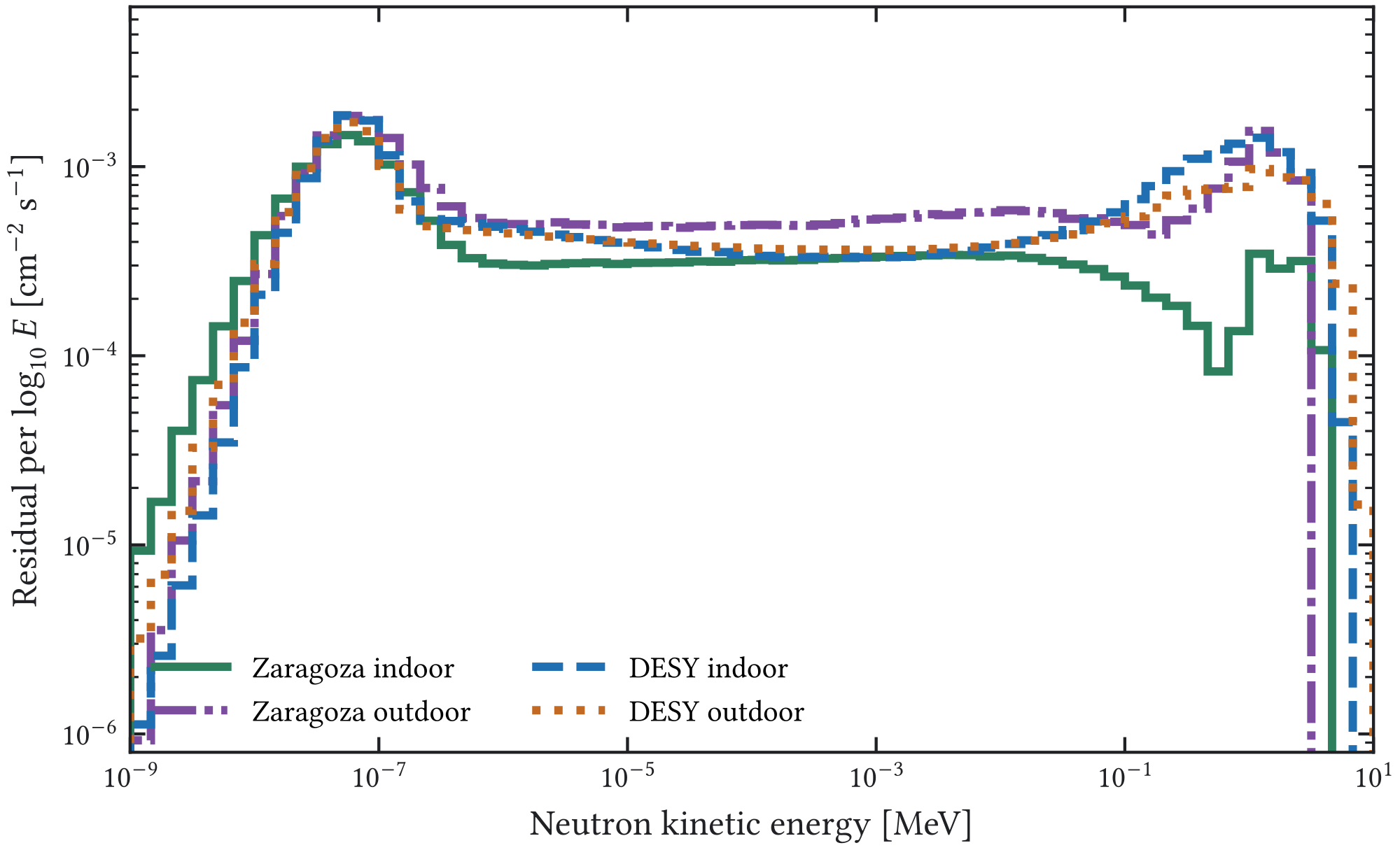
The processed residual-neutron statistics combine the original sparse residual pass with the closed-pipe extension completed on 14 May 2026. After detector reconstruction, 703 indoor-residual events and 626 outdoor-residual events are available for the selection study. The final X-ray-like selection is still limited by one indoor event and zero outdoor events, so the last rows of Table 6.15 should still be interpreted with finite-statistics confidence intervals rather than as precise rate measurements.
6.5.1.5 Current detector-level results
Table 6.15 and Figure 6.10 summarize the current detector-level environmental-background estimates in the – reference window. The selections are applied progressively: first the fiducial reconstructed energy window, then a basic topology preselection, and finally the legacy X-ray-like cuts used for this environmental-response comparison. These rows have not yet been rescored with background-analysis-v2-conservative-reference and are therefore auxiliary site-transfer estimates rather than entries in the partial inventory.
| Source | Selection | Events | Background level with 90% C.I. |
|---|---|---|---|
| Environmental gammas | Fiducial energy | 18 | |
| Environmental gammas | Fiducial + topology preselection | 2 | |
| Environmental gammas | X-ray-like cuts | 0 | |
| Indoor residual neutrons | Fiducial energy | 229 | |
| Indoor residual neutrons | Fiducial + topology preselection | 27 | |
| Indoor residual neutrons | X-ray-like cuts | 1 | |
| Outdoor residual neutrons | Fiducial energy | 200 | |
| Outdoor residual neutrons | Fiducial + topology preselection | 16 | |
| Outdoor residual neutrons | X-ray-like cuts | 0 |
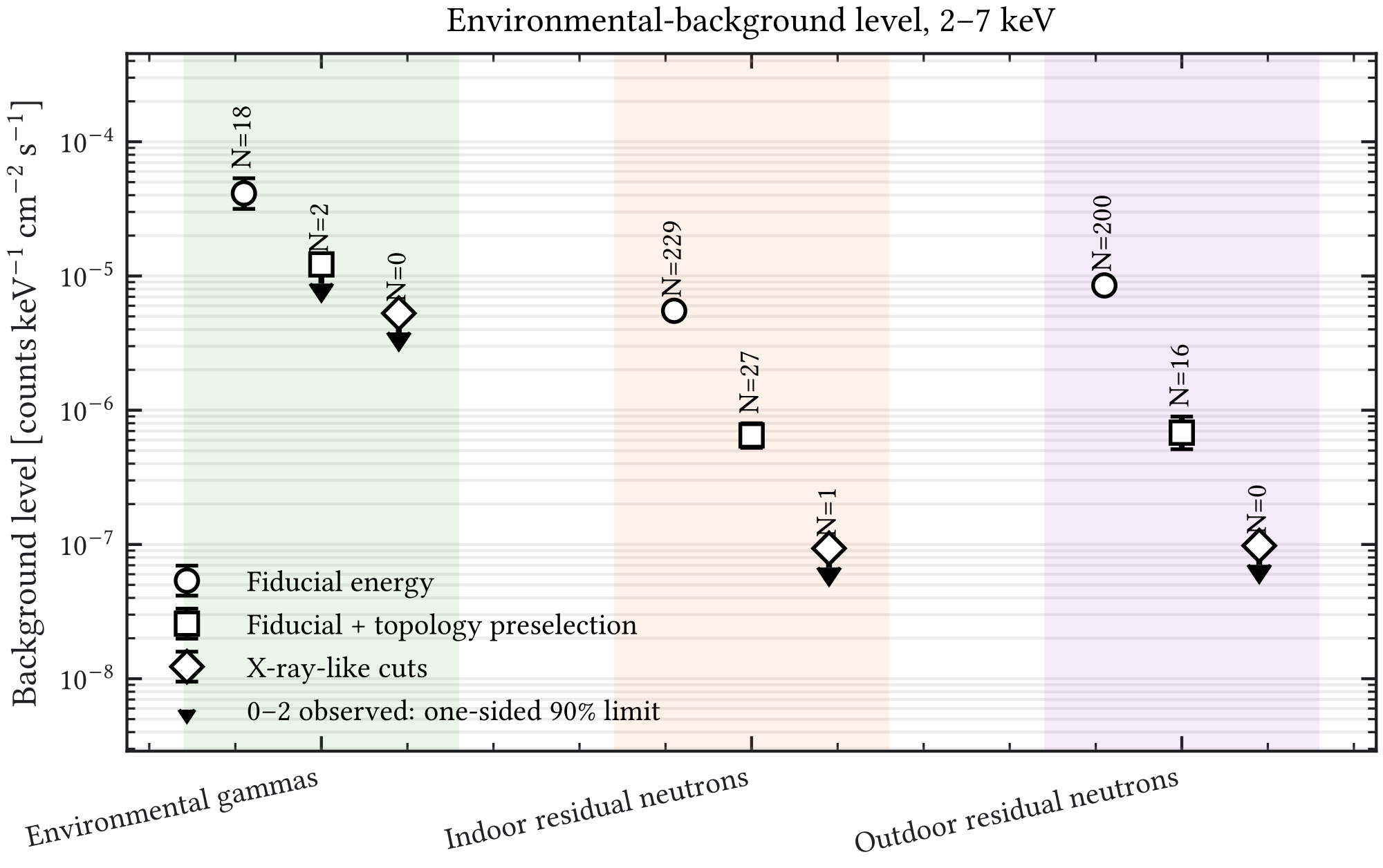
The NaI-normalized environmental-gamma sample has no event after the legacy X-ray-like selection, giving the exposure-limited bound at 90% confidence. Because this bound is above the intended background scale and the selector is legacy, the result does not establish that environmental gammas are negligible. The indoor residual-neutron sample has one selected event and is reported as at 90% confidence. The outdoor residual-neutron sample is presently only an upper limit after cuts, at 90% confidence. The main systematic limitation for both source components remains the site normalization: the gamma field should ultimately be replaced by a DESY-specific measurement or radiation map, and the residual-neutron spectra should be revisited once the selected BabyIAXO site and its boundary conditions are fixed.
6.6 Cosmic-ray background
The surface operation of BabyIAXO makes cosmic-ray secondaries a central part of the external-background model. The relevant components are muons, neutrons, protons, gamma rays, and electrons/positrons. They are treated as separate source components because their spectra, angular distributions, detector-facing rates, and veto signatures are physically different. Muons are the dominant penetrating charged component at ground level and are expected to be controlled mainly by the prompt active veto. Neutrons are the most subtle component: they are neutral, penetrate shielding efficiently, and can produce low-energy Micromegas deposits through hadronic cascades, capture or de-excitation photons, electromagnetic descendants, and delayed activation products. Cosmic gamma rays, electrons/positrons, and protons are expected to be subdominant, but they are included to close the surface-cosmic source inventory and to test whether non-muon, non-neutron atmospheric secondaries can populate the – Micromegas region after detector-response processing.
The source-yield comparison uses the deterministic energy, one-track, and maximum-track-center definition for Guan muons, the three light CRY components, and both timing channels of the HENSA outdoor-neutron field. The 249 selected neutron histories are joined to their transport ancestry, separating 246 prompt/non-delayed candidates from three delayed activation events. A higher-statistics historical sample supplies supplementary mechanism diagnostics. The learned topology selector is not credited, while deterministic reconstruction and fiducial acceptance remain conditional on the simulated detector response. Campaign exposure and source-angle conventions must close independently before these yields become absolute rates. Appendix Section A.8 records the preserved generated and selected event counts.
6.6.1 Cosmic source components and normalization
Cosmic-ray source terms are normalized at the level of generated primaries rather than at the level of saved or reconstructed events. For an incident component with generated-primary rate , the detector-level background level after a selection is computed as
(6.8)
where is the number of generated primaries, is the number of reconstructed events surviving the selection, for the – reference window, and is the detector area associated with that selection. This convention keeps the physical source normalization independent of the detector-response filtering and of the number of events saved by restG4. For the current cut-flow tables, the pre-fiducial rate stages use the full readout area, , because no central-radius requirement has yet been applied. Beginning with the fiducial column, the normalization area is the -radius axion-window region, .
For the muon sample, integration of the Guan parametrization over and the downward hemisphere, with applied once, gives a scalar fluence rate of [104]. Its conversion to generated primaries requires the projected generation surface of each campaign. The historical cut-flow calculation used , whereas a read-only check of one preserved May 17 campaign file records . These surfaces cannot be interchanged: the former reproduces the previously quoted muon exposure, but does not establish the exposure of every archived file. The results below therefore report selected-event yields per generated primary; no absolute muon bound is inferred from either unverified surface choice. The local Guan source configuration also emits only negative muons. Although penetrating energy loss is similar for the two charges, stopping negative-muon capture changes neutron and activation production, so a charge-composition check is required before interpreting the sample as the complete field.
The neutron energy distribution originates from the outdoor HENSA unfolding extending to [126]. The production configuration restricts incident neutrons to energies above ; lower-energy descendants are transported, but lower-energy incident neutrons are a separate source contribution. HENSA constrains an energy-dependent scalar fluence, not an angular distribution. The assumed downward law must therefore be distinguished from the measured spectrum and from a horizontal crossing distribution. The historical Cosmics adapter divides histogram bins by the cosine of the zenith-bin center. Applied to a scalar-fluence histogram without compensating encoding, this changes the continuous angular law to and increases its integral by a factor of . Consequently, an angular correction requires event weights or new transport; dividing every surviving background level by would ignore the angle dependence of shielding and veto response.
An explicit source-construction check separates bin-integrated fluence from densities in or , encodes the inverse-cosine adapter, and preserves the input and output hashes. For an isotropic scalar field , the sphere crossing rate is ; a horizontal plane instead receives . The new generator-only geometric check reproduces the plane/sphere crossing ratio within standard deviations in trials. An independent check of the installed REST source reader restores every candidate histogram bin within relative precision and samples neutrons both with and without the restriction. The sampled restricted-range acceptance, 0.51496, agrees with the histogram integral, 0.51409, and the unrestricted mean agrees with the declared angular law. This verifies the declared sampling convention, without replacing the missing archived-source provenance or validating the physical HENSA angular field. The preliminary DESY unfolding also retains pressure, solar-modulation, noise-selection, and unfolding-prior uncertainties [127]. For gamma rays, protons, and electrons/positrons, CRY is used as the current surface-cosmic source model.
| Component | Source term | Detector-facing generation | Current quantitative use | Main remaining limitation |
|---|---|---|---|---|
| Guan muons | Guan sea-level muon formula | Detector-facing REST cosmic surface; prompt charged tracks through shielding and veto | Deterministic pre-veto yield bound; absolute exposure unresolved | Independent Monte Carlo exposure, geometry, and site validation |
| Outdoor HENSA, generated above to | Surface neutron source transported through lead, cadmium, scintillator, and detector materials | Generated-event yields and causal prompt/activation split; legacy veto diagnostic | Source transfer to DESY, veto-response domain transfer, hadronic model dependence, and delayed activation statistics | |
CRY surface gamma rays | Neutral electromagnetic component; Micromegas deposits arise through secondary charged particles | Deterministic pre-veto selected-event yield | Final site spectrum and exposure | |
CRY surface electrons and positrons | Charged electromagnetic component with short penetration length and bremsstrahlung secondaries | Deterministic pre-veto selected-event yield | Sparse fiducial statistics and final surface-source validation | |
CRY surface protons | Charged hadronic component; cascades resemble neutron-induced secondaries but usually with prompt veto activity | Deterministic pre-veto selected-event yield | CRY source-model dependence and finite fiducial statistics |
6.6.2 Gamma-ray, electron, and proton mechanisms
Dedicated CRY configurations were prepared for surface photons, electrons/positrons, and protons. These components are retained to close the surface-cosmic source inventory and to test different routes to a low-energy Micromegas deposit. Cosmic gamma rays are neutral at generation, so they contribute to the Micromegas only after Compton scattering, pair production, or an electromagnetic shower in the shielding or detector materials. Electrons and positrons are charged and can produce prompt veto activity, but they also radiate bremsstrahlung photons that initiate secondary electromagnetic deposits. Protons are charged hadrons; if the primary or a charged secondary reaches the scintillator system it tends to give a prompt high-ionization veto response, while the hadronic cascade itself remains a useful control sample for neutron-like secondary production.
Truth-history classification confirms that gamma- and electron-induced TPC deposits are overwhelmingly electromagnetic: in the higher-statistics gamma diagnostic, secondary electrons or positrons dominate of events with a non-zero Micromegas signal. The proton response is more mixed, combining electromagnetic descendants with proton recoils, charged cascade particles, neutrons, and nuclear fragments. The detailed classification, detector-response cut flow, and representative event displays are retained in Appendix Section A.9. These diagnostics support the mechanism interpretation, but none supplies topology or veto-rejection credit to the conservative reference.
6.6.3 Current cosmic-ray cut flow
Table 6.17 reports the selected-event yield per generated primary after the common energy, one-track, and fiducial requirements. This quantity isolates the reconstructed response from the unresolved conversion of incident phase space to physical exposure. The samples use the -tuned reconstruction; agreement of that response with the relevant detector data remains a separate uncertainty even though no learned topology rejection is credited.
| Source | Generated primaries | Selected | Selected-event yield |
|---|---|---|---|
| CRY | 1 | ||
| CRY | 1 | ||
| Guan muons | 0 | ||
| HENSA , aggregate | 249 | ||
| prompt/non-delayed | 246 | ||
| delayed activation | 3 | ||
| CRY | 44 |
No muon event survives the fiducial requirement in the -primary sample. The corresponding event-yield upper bound is per generated muon at 90% confidence. The track-position diagnostic in Appendix Section A.9 explains this rejection, but a bound in physical background units requires the campaign-specific area and source normalization described above. Further muon production should follow that normalization check and a charge-composition control. The absence of a delayed ancestor in the audited muon survivors is not evidence that muon-induced activation is identically zero.
The legacy prompt-veto overlay applied to the 246 prompt neutron candidates leaves 22 entries in its first fixed draw, with a central 90% population range of 19–25 across 200 overlays. These counts illustrate sensitivity to accidental activity; they do not establish a physical-window-corrected neutron rejection efficiency. The acquisition-window and calibrated-energy qualifications in Section 5 apply before such a veto factor can enter the physical background model. The full historical topology/veto cut flow remains an auxiliary diagnostic in Appendix Section A.9.
6.6.4 Cosmic-ray event classes and veto survival
The source-by-source background rates do not fully describe how cosmic-ray events appear after reconstruction. For the background model, however, the role of the detailed event-history studies is deliberately limited: they diagnose why any future validated survival treatment must remain source and timing-channel dependent. The detector-level interpretation of prompt muon tags and late-window neutron-sensitive observables, together with the comparison with experimental IAXO-D0 veto data, is given in Section 5. The truth-history classification used to support that interpretation is presented in Figure 6.6 of Section 5.
The relevant distinction is that cosmic-ray sources do not survive the analysis for the same physical reason. Muon-induced events usually carry a prompt, high-amplitude, multi-panel scintillator signature. Their residual contribution after the prompt veto is therefore expected to be dominated by atypical cases: inefficient regions, unstable or disabled channels, weak prompt deposits, or secondary particles produced by the muon in the surrounding materials. Neutron-induced events are less direct. The neutron-history study in Figure 6.6 shows that the largest class of TPC-depositing neutron events is produced by electromagnetic descendants rather than by a primary neutron scattering elastically in the gas. This explains why a neutron-initiated event can look X-ray-like in the Micromegas while still leaving late-window, multiplicity-rich, or spatially diffuse veto activity in the scintillator–cadmium system. There is also a delayed-activation tail in which the neutron produces an unstable residual nucleus and the low-energy TPC event occurs only when that product decays. This channel is not mitigated by tightening the veto selection, because the correlated scintillator activity belongs to the original neutron interaction rather than to the later Micromegas trigger. The dedicated discussion in Section 6.7 quantifies this effect under the conservative reference and retains the larger legacy sample only as a mechanism diagnostic. The apparent reduction of the delayed channel by the legacy Micromegas topology selector is not credited in the conservative result.
This separation keeps the background-model chapter focused on the source inventory and rate construction. The veto observables enter here as reconstructed selections and efficiencies, not as truth-level labels. Consequently, each rate should be read under the explicitly documented Micromegas selector and source-dependent veto treatment. A conservative-reference prediction is the target of the registry, not an assumption applied retrospectively to the legacy rows. The event-history diagnostics remain essential, but their detailed presentation is retained in Appendix Section A.5, where truth-level mechanisms are kept separate from the source-normalized rate accounting presented here.
6.6.5 Cosmic-induced veto activity and random coincidences
The same surface-cosmic simulations can also be used to estimate the rate of veto activity that is unrelated to an otherwise signal-like Micromegas trigger. This contribution is not a background level in the Micromegas region of interest. It supplies an accidental-veto input for estimating the chance coincidence of unrelated activity with an X-ray-like event. The relevant quantity is therefore the visible veto-trigger rate, defined here as the rate of simulated cosmic events with at least one reconstructed rawPeaksVETO peak after the full detector-response chain. This definition includes the same quenching, light attenuation, waveform shaping, digitization, baseline correction, and peak threshold used for the background cut flow. Events with no reconstructed veto peak are not counted as veto-noise triggers, because they would not be observable as veto activity in the analysis.
Dedicated veto-noise productions were generated for muons, neutrons, gammas, protons, and electrons/positrons, with the TPC and veto scintillators treated as sensitive volumes. The normalization uses the equivalent physical time of each generator sample, while the numerator counts only events with at least one reconstructed veto peak. Approximating each visible event as a point trigger with independent Poisson arrivals gives the probability of at least one trigger in a window :
(6.9)
where is the event rate, not the rate of individual peaks. For a correlated peak train of finite duration, the probability that any peak overlaps a randomly placed window also depends on the train timing; the point-trigger approximation does not capture that effect. Table 6.18 summarizes the current rate estimate.
| Source | Triggers | Time [s] | Rate [Hz] | [%] | [%] |
|---|---|---|---|---|---|
| Muons | 97443 | 266.21 | 3.59 | 30.7 | |
| 65908 | 1372.31 | 0.479 | 4.69 | ||
| 36094 | 601.18 | 0.599 | 5.83 | ||
| 38415 | 949.75 | 0.404 | 3.96 | ||
| 68166 | 24328.40 | 0.0280 | 0.280 |
rawPeaksVETO peak after detector-response processing. The muon exposure includes the correction for the duplicated azimuth factor in the legacy Guan metadata, identified by its stored flux; its generation area is unchanged. The last two columns give the point-trigger Poisson occupancy for windows of and ; extended correlated peak trains require a timing-overlap calculation.The muon component dominates the accidental-veto rate because the surface muon flux is large and almost every saved muon event produces a reconstructed veto peak. The other components are much smaller, although gamma, electron/positron, and neutron primaries still produce visible veto-trigger rates at the level of tens of hertz in the present detector-facing geometry. The proton rate is lower after normalization to the generated physical time, despite the large fraction of proton events with visible veto activity.
Table 6.18 gives point-trigger occupancies, not rejection or dead-time probabilities for the published veto logic. They approximate signal loss for a rule that rejects any visible activity only when the point-trigger treatment is adequate; an operational efficiency requires the full peak or waveform timing, coincidence logic, and measured channel state.
Peak multiplicity, energy sharing, and panel occupancy are retained as supporting detector-topology diagnostics in Appendix Section A.2, Figure A.14 and Figure A.16; they do not enter the absolute rate normalization. In particular, no peak-multiplicity requirement is applied to the rates or accidental occupancies reported here. Multiplicity is a diagnostic input to the separately calibrated multivariate veto selections described in Section 5, not a frozen standalone operating criterion.
Figure A.15 converts the visible veto-trigger rates into accidental probabilities over the full coincidence-window range. For short windows of order , all non-muon components remain below the percent level. At , the corrected muon-induced occupancy is , while the other components remain below . At , the muon occupancy reaches . This behavior is a useful reminder that the veto selection has two different effects: it rejects correlated cosmic backgrounds, but it also introduces an accidental live-time or signal-efficiency cost that depends directly on the chosen time window and on the visible veto-trigger rate.
6.7 Neutron-induced activation background
The selected veto geometry, including the cadmium sheets placed between plastic-scintillator stages, is defined in Section 5; that chapter also establishes the lead-cascade, moderation, prompt-recoil, and cadmium-capture mechanisms. For the background model, their principal consequence is an accounting rule: a prompt veto selection cannot be applied indiscriminately to every neutron-induced event.
The outdoor HENSA field is therefore partitioned into prompt, non-delayed histories and delayed-activation histories. In the latter, a neutron activates a nucleus in the detector or shielding and the Micromegas signal is produced by a later radioactive decay. The original interaction may produce veto activity, but the decay can occur long after the recorded coincidence window and therefore cannot receive prompt-veto credit. The delayed channel remains a separately normalized residual unless a validated Micromegas selection removes it.
The delayed-decay label is assigned from the saved Geant4 event history by following the parent chain of the gas energy deposits and requiring a RadioactiveDecay step more than after the primary neutron interaction. The diagnostic cut flow, activation-product distribution, and representative delayed and prompt no-veto survivor displays are retained in Appendix Section A.5. For the rate model, the controlling point is that prompt-veto rejection cannot be assigned to the delayed branch.
The archived HENSA productions already transport the full hadronic and radioactive-decay chain, including the residual nucleus, its decay time, and the detector response of its descendants. The conservative-reference history audit therefore reuses the exact 249 detector-level candidates in Table 6.17 rather than introducing a second transport sample. For each candidate, every track depositing energy in the TPC gas is followed through its causal ancestry. Only a radioactive decay in that ancestry is classified as activation; an unrelated delayed decay elsewhere in the same simulated event is insufficient. The boundary matches the subevent separation used in the production and is beyond the prompt coincidence regime considered for the neutron-sensitive veto. It is an analysis boundary between detector timing channels, not a definition of nuclear activation.
That detector-coupled audit is complemented here by an unbiased production inventory. The inventory calculation retained every primary and every residual-nucleus track, irrespective of whether the event later deposited energy in the TPC. One hundred independently seeded jobs generated incident neutrons and inspected Geant4 tracks. The historical exposure was parsed from a restG4 summary that divided by the full spectral integral without the configured energy-range acceptance. It is therefore not used here as a physical irradiation time. The inventory instead reports yields per generated neutron; converting these to production rates requires the corrected, campaign-specific source ledger. The residual-nucleus ledger contains direct or secondary products and keeps them separate from radioactive-decay descendants, thereby avoiding double counting a parent and its simulated daughter chain.
Table 6.19 summarizes representative products with operationally relevant half-lives. These are production counts, not selected background events. In particular, the campaign produced 124 nuclei, corresponding to a central yield of products per generated neutron. This supports an isotope-level comparison within the simulated incident phase space; source-field and hadronic-model uncertainties remain separate from the counting precision. However, is not the most frequently produced radionuclide: is produced approximately 24 times more often, and several lead, cadmium, and veto-material products also have larger yields. The background relevance of depends on both production and detector coupling, while its long half-life determines buildup and persistence during cooldown.
| Product | Count | Yield per | Half-life | Main production region |
|---|---|---|---|---|
| 6241 | 4487.5 | Lead shielding | ||
| 3014 | 2167.2 | Copper box, detector pipe, and chamber | ||
| 2348 | 1688.3 | Carbon-bearing plastic-veto volumes | ||
| 1164 | 837.0 | Cadmium neutron-capture layers | ||
| 698 | 501.9 | Plastic-veto and light-guide volumes | ||
| 671 | 482.5 | Cadmium neutron-capture layers | ||
| 149 | 107.1 | Copper box and detector pipe | ||
| 124 | 89.2 | Copper box and detector pipe | ||
| 104 | 74.8 | Copper box and detector pipe |
Geant4 11.0.3 radioactive-decay data used for transport. The table is not a complete ranking by raw residual-nucleus count: effectively stable products and very rare products are retained in the machine-readable inventory but omitted here.For a constant production rate , zero initial inventory, retention in the production volume, and subsequent source-off cooldown, the activity of isotope is
(6.10)
At saturation, , independently of the half-life. Decay-chain feeding requires a coupled Bateman calculation; for a well-mixed flowing gas, removal adds to the loss rate, where is the volumetric flow and the active volume. Initial cosmogenic contamination must be included as an initial inventory rather than counted again in the ongoing production term.
The decay-response calculation then generates each radionuclide at rest and uniformly within its observed production volume in the exact IAXO-D1 geometry. Repeated veto logical volumes are represented by six deterministic, approximately uniformly spaced physical placements. The complete radioactive chain, low-energy electromagnetic transport, atomic relaxation, REST detector response, and standard reconstruction are applied before the same conservative –, one-track, and fiducial selection used in Table 6.17. No prompt-veto rejection is applied.
The broad response screen includes every isotope–volume pair with at least 20 direct products, every pair in the gas or a detector-adjacent volume irrespective of its observed yield, and a set of long-lived priority products. It represents 194,581 of the 197,681 direct radioactive products in the inventory, or 98.4%, through 332 logical pairs and 769 physical source placements. Twelve source jobs in distant scintillator volumes terminated inside the Geant4 radioactive-decay transport; the remaining 757 jobs, covering 330 logical pairs, completed normally. This missing branch represents 156 production tracks and is retained as a small, explicitly unmodeled tail rather than assigned zero background.
The short screen generated radioactive decays. Of these, 322 produced a saved TPC event, 321 entered the reconstructed feature tree, 75 satisfied the – and full-readout requirements, 50 also had one track in each projection, and none satisfied the final fiducial requirement. This result shows that detector coupling, rather than radionuclide production, controls the required decay statistics. The component-wise bounds from the screen were therefore used only to allocate a high-multiplicity follow-up to the pairs that dominated continuous-saturation and five-year-plus-cooldown scenarios. Finite irradiation and cooldown scenarios are obtained by weighting each source response with Equation (6.10).
The follow-up comprised 3,000 jobs allocated by the five-year-plus-cooldown ranking, 1,750 jobs allocated by the saturation ranking, 500 jobs covering every observed production volume, and 450 jobs covering every observed production volume. Every job completed successfully. Together with the broad screen, these campaigns generated radioactive decays, of which 79,007 produced a saved TPC event, 78,678 entered the reconstructed feature tree, 17,433 passed the energy and full-readout requirements, 9,441 also passed the one-track requirement, and 73 satisfied the final fiducial selection. The selected sample contains 54 decays and 19 decays; no other screened isotope survived the complete selection.
The observed decay responses can be combined with production counts without assigning an unverified physical exposure. Define the selected-event yield per generated incident neutron as
where is the simulated decay-selection response for isotope in volume . The central saturation yields are for and for per generated incident neutron. Their sum is a production-volume model result for the sampled phase space, not an upper limit on every activation product. Once the incident rate is established, the corresponding background level follows from .
| Scenario | Combined selected-event yield | ||
|---|---|---|---|
| 30 days, no cooldown | 0.2543 | 0.0107 | |
| 1 year, 1-day cooldown | 0.9625 | 0.1232 | |
| 5 years, 30-day cooldown | 0.7457 | 0.4767 | |
| Saturation, no cooldown | 1.0000 | 1.0000 |
dominates the finite irradiation scenarios through five years followed by a 30-day cooldown. supplies approximately 56% of the modeled saturation yield because of the product of production yield and detector coupling, and its half-life makes that activity persist during cooldown. Coverage of 98.4% of produced radioactive nuclei does not imply the same coverage of accepted background: a rare product near the gas can couple more efficiently than a common product far away. The omitted isotope-volume tail and the six-placement approximation therefore require response-weighted bounds. The component-wise statistical envelopes are not a joint 90% interval. Bonferroni-adjusted isotope intervals are conditional on valid production and response marginals; cascade correlations and pilot-directed allocation must be included before asserting unconditional coverage.
The detector-coupled ancestry study provides a complementary result that preserves the actual production positions of the selected histories. Three of the 249 candidates are delayed activation: two decays following capture in copper and one decay following capture in argon. The remaining 246 histories are prompt or non-delayed, as shown in Table 6.17. For the separate delayed-channel bound, a predeclared one-sided 90% construction gives a selected-event-yield limit of per generated incident neutron under the simulated decay and selection assumptions. This conditional bound does not cover an ungenerated low-energy incident field or an unmodeled isotope response.
| Product | Production region and process | Half-life | Selected |
|---|---|---|---|
| Neutron capture in copper chamber body/backplate | 2 | ||
| Neutron capture in the argon-based gas | 1 |
Geant4 11.0.3 decay data used for transport. This selected-event inventory is distinct from the inventory of all nuclei produced in the geometry.| Scenario | Effective selected decays |
|---|---|
| 1 day, no cooldown | 2.460 |
| 30 days, no cooldown | 3.000 |
| Saturation, no cooldown | 3.000 |
| Saturation, 7-day cooldown |
Both selected products are effectively saturated after 30 days of continuous irradiation in the retained-inventory model; after one day, their combined response reaches 82% of saturation. Longer-lived cobalt contributions are characterized by the dedicated volume study rather than inferred from their absence among three rare selected histories. Delayed activation remains a distinct source class with no prompt-veto rejection credit.
The higher-statistics legacy HENSA-neutron response audit is summarized in Table 6.23. The table reports the prompt non-delayed residual and delayed-activation upper limit as separate channels. The delayed branch is evaluated after the fiducial – and full TPC/X-ray topology selections, but without crediting any prompt veto rejection. The non-delayed branch uses the complete prompt selection chain: fiducial – readout energy, veto ML, X-ray BDT, and reconstructed-hit fiducial containment. In the photon-evaporation HENSA-neutron sample, the delayed component has no surviving events after the full Micromegas topology and reconstructed-hit fiducial selections, so it is retained as a separate confidence upper bound.
| Neutron component | Selection stage | with 90% interval or upper bound | |
|---|---|---|---|
| All neutron-induced events | Fiducial – | 124328 | |
| All neutron-induced events | Fiducial – + veto ML | 22858 | |
| All neutron-induced events | Fiducial – + full TPC/X-ray selection; no veto cut | 63 | |
| Delayed activation | Fiducial – + full TPC/X-ray selection; no veto cut | 0 | |
| Non-delayed prompt tail | Fiducial – + full TPC/X-ray selection; no veto cut | 63 | |
| Non-delayed prompt tail | Fiducial – + veto ML + full TPC/X-ray selection | 16 |
readoutEnergyInFiducial, reconstructed-hit-centroid containment, and , rather than the conservative-reference maximum-track definition in Table 6.2 and area. The all-event rows show the cumulative neutron reduction before the delayed/non-delayed split is applied. The delayed contribution is defined without applying a prompt veto cut, because delayed activation is not a prompt-coincidence topology. The non-delayed component is evaluated with the prompt veto ML selection in its last row. Ordinary-count rows use central Garwood intervals propagated through the common neutron-source normalization; the zero-survivor delayed row is a one-sided upper bound. No combined confidence interval is constructed: the prompt central interval and delayed zero-count bound remain separate until a joint statistical construction is defined.Under the stricter legacy full Micromegas topology and reconstructed-hit fiducial-containment requirement, the delayed-activation component has no survivor. It is nevertheless kept as a separate upper-limit component because the prompt veto cut cannot be credited for rejecting it. The legacy response scale is therefore reported as two statements: and , without combining them into a nominal 90% interval. These historical rate values retain their original source normalization and selector assumptions; neither has been promoted to an absolute current bound. The generated-event yields above provide the exposure-independent comparison.
6.8 Cosmic and activation background status
The quantitative cosmic result is the source-yield inventory in Table 6.17. Its six leaf channels retain the deterministic reference selection and their generated-primary denominators. The prompt-neutron overlay remains a conditional legacy veto diagnostic: the stored observables do not permit the full calibrated-energy feature to be recomputed in a corrected physical time window. No absolute post-veto background rate is credited, and delayed activation receives no prompt-veto rejection. The higher-statistics results in Table 6.23 are retained only for mechanism interpretation and historical accounting.
6.9 Status and uncertainty roadmap
The quantitative endpoint of this chapter is a partial IAXO-D1 argon source-response model under the deterministic contract in Table 6.2. It includes an incident-photon-denominator signal response, generated-primary cosmic yields, a separate time-dependent activation model, a 30-source provenance registry, and explicit statistical reporting conventions. Absolute source-rate promotion requires matched campaign ledgers and detector-response validation. A closed total additionally requires compatible intrinsic, material, environmental, and telescope-side responses with detector-specific normalization and complete source support. The BabyIAXO Xe–Ne detector, telescope optics, final veto, and DESY source terms constitute a separate projection and are not mixed with the IAXO-D1 reference.
| Source | Input normalization | Geometry / setup | Analysis treatment | Dominant uncertainty | Status |
|---|---|---|---|---|---|
| Gas and radon | Gas composition, radon assumptions, screening inputs | Active gas volume and detector chamber | Legacy transparent topology branch | Concentration, plate-out, emanation history, conservative-reference rescoring | Stored response counts available; generated-parent normalization and reference rescoring required |
| Materials, electronics, and shielding | Radiopurity screening and component masses | Source-specific detector volumes | Mixed legacy energy-binned, BDT, and fiducial definitions | Screening limits, geometry details, selection harmonization | Several reusable transports; no conservative-reference material sum |
| Telescope-side optics/pipe | Optics or pipe activity assumptions | BabyIAXO telescope-side generator volume | Cone-biased photon transport; pilot response and production audit only | Geometry realism, activity vector, incomplete reprocessing | Separate BabyIAXO projection |
| Environmental gammas | Laboratory spectra and concrete simulations | Room model around detector | Transport to detector and Micromegas selection | Site dependence and material composition | Awaiting DESY-specific source term |
| Environmental neutrons | Literature/model inputs and local measurements | Laboratory neutron field around shielding | Legacy detector-response selection | Source normalization, moderation model, selector, and DESY transfer | Auxiliary residual estimate |
| Cosmic muons | Guan sea-level CosmicMuons model, with CRY cross-checks | Surface detector with shielding and veto | Contract-compatible deterministic reference, pre-veto | Exposure, geometry, and site transfer | Generated-primary yield bound; exposure unresolved |
| Cosmic protons | CRY surface source term | Surface detector with shielding and veto | Contract-compatible deterministic reference, pre-veto | Finite statistics and site transfer | Generated-primary yield; exposure unresolved |
| Cosmic neutrons | HENSA outdoor 10 GeV spectrum, with CRY/EXPACS cross-checks | Surface detector with lead and veto volumes | Deterministic prompt/non-delayed and activation yields; conditional legacy veto overlay | DESY transfer, veto-response domain transfer, and hadronic modeling | Leaf yields available; source and response validation open |
| Conservative-reference disposition | Sources | Meaning |
|---|---|---|
| Available deterministic response | 4 | Guan muon and three CRY light-particle rows already provide the exact pre-topology, pre-veto response. |
| Reprocess preserved output | 11 | Required reconstructed branches or events exist; apply the conservative reference before new transport. |
| Resolve source normalization | 8 | A response or transport basis exists, but a detector-specific activity, site field, or scenario choice is missing. |
| Define source model or geometry | 7 | New transport is justified only after the physical source term and relevant detector volume are specified. |
background-analysis-v2-conservative-reference. The categories are mutually exclusive and exhaustive. Four deterministic responses are available for the partial inventory, but the unresolved rows preclude an unconditional total.The selector-incompatible historical response scale is retained in Appendix Section A.6. It identifies the physical mechanisms and normalization assumptions retained from the earlier source studies; invalid parent-decay conversions are omitted, and incompatible scenarios and selections are not summed. The scientifically defensible endpoint is therefore the conservative IAXO-D1 partial inventory together with the explicit open-component dispositions, not a single BabyIAXO background level.
The next quantitative step does not depend on finding another topology classifier. Work that can proceed without new physics input includes conservative-reference reprocessing of seven preserved source samples, source-specific validation of the prompt-neutron veto response, and regeneration of the partial inventory from machine-readable outputs. Closing the absolute IAXO-D1 inventory then requires detector-specific choices or measurements for the sixteen normalization-blocked sources and physical definitions for the seven source-model or geometry rows. The detailed analysis and source-model roadmap is retained in Appendix Section A.7; veto-specific uncertainties remain in Section 5. The BabyIAXO Xe–Ne, optics, final-veto, and DESY-site calculation must be constructed afterward as a separate contract rather than as an implicit correction to the argon reference. For each included source, the collaboration table should record the input normalization, geometry and configuration hashes, exposure or number of primaries, analysis identifier, surviving level, statistical interval, systematic uncertainty, and inclusion status. The registry and conservative contract make that extension auditable and prevent an omitted or incompatible component from being silently interpreted as zero.