Experimental Typst web edition · Veto chapter pilot

2 The Helioscope Technique and the IAXO Program

Introduction

Solar helioscopes combine a well-characterized astrophysical source with magnetic conversion and a tracking-correlated X-ray signal. This chapter develops the signal yield and statistical sensitivity, then follows the progression from CAST to the International Axion Observatory (IAXO) and its intermediate stage, BabyIAXO [13, 14, 46]. The connection to the present work is the detector-background requirement: a larger magnetic aperture is useful only if the optics and detector retain the converted photons while suppressing the background collected with them. Published design projections, the March 2026 engineering and site studies, and the subsequent funding milestone are distinguished below; the project-status cutoff is September 2026.

2.1 The Helioscope Technique

2.1.1 Solar Axions

Solar axions are produced in the hot, dense plasma of the Sun through several processes. The best known is Primakoff conversion, in which thermal photons convert into axions in the electromagnetic fields of charged plasma constituents. Additional contributions arise from processes involving the axion–electron coupling: atomic axio-recombination and axio-deexcitation, electron–ion and electron–electron bremsstrahlung, and Compton-like scattering. These processes are commonly grouped as the ABC channels [27].

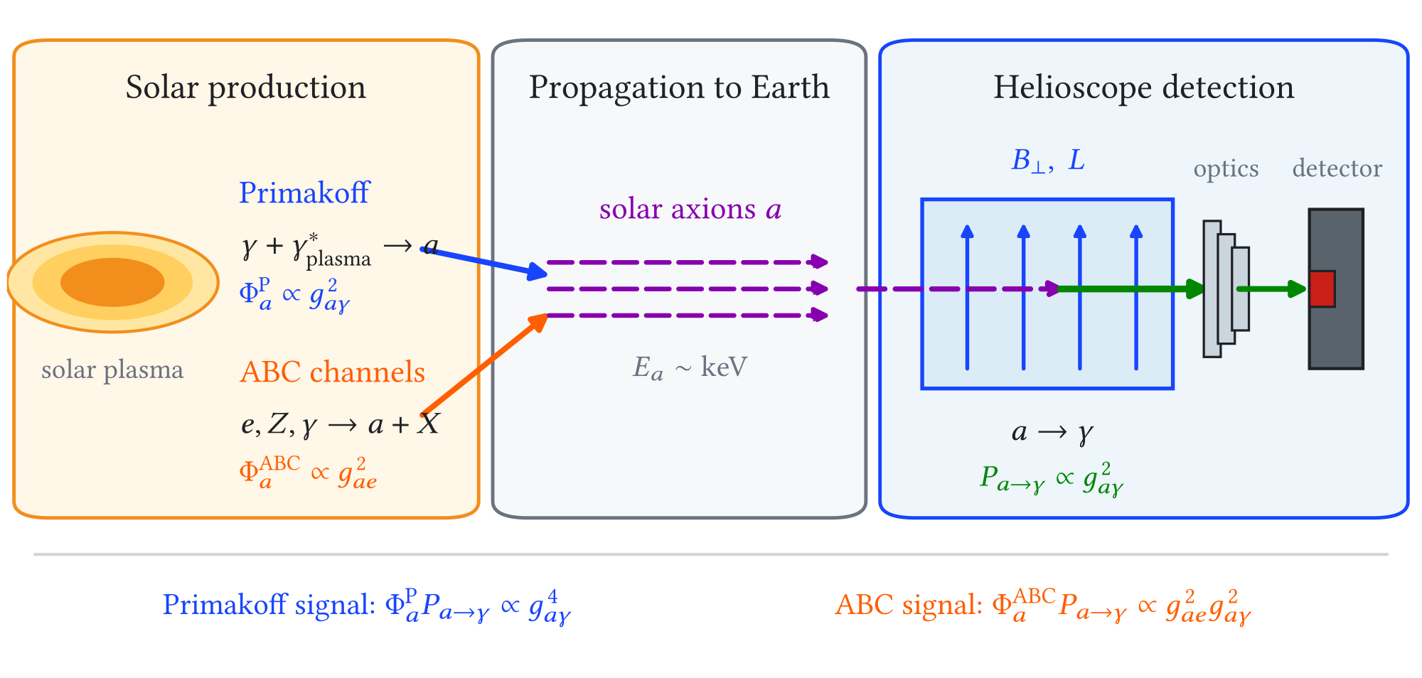
Figure 2.1: Schematic production and detection chain for solar axions in a helioscope. Primakoff production in the solar plasma is controlled by 𝑔 𝑎 𝛾 , whereas ABC production is controlled by 𝑔 𝑎 𝑒 . Detection in the magnet occurs through inverse Primakoff conversion and therefore depends on 𝑔 𝑎 𝛾 . — Figure 2.1: Schematic production and detection chain for solar axions in a helioscope. Primakoff production in the solar plasma is controlled by $𝑔_{𝑎 𝛾}$ , whereas ABC production is controlled by $𝑔_{𝑎 𝑒}$ . Detection in the magnet occurs through inverse Primakoff conversion and therefore depends on $𝑔_{𝑎 𝛾}$ .

The coupling dependence follows directly from this chain. For Primakoff solar axions, both production in the Sun and conversion in the laboratory depend on $𝑔_{𝑎 𝛾}$ , so the expected signal rate scales as $𝑔_{𝑎 𝛾}^{4}$ . For ABC solar axions, production depends on $𝑔_{𝑎 𝑒}$ , whereas detection still requires axion–photon conversion, so the signal rate scales as $𝑔_{𝑎 𝑒}^{2} 𝑔_{𝑎 𝛾}^{2}$ . Primakoff data therefore constrain $| 𝑔_{𝑎 𝛾} |$ , whereas ABC data constrain the product $| 𝑔_{𝑎 𝑒} 𝑔_{𝑎 𝛾} |$ . Separating the two couplings requires an additional model assumption or an independent constraint.

Figure 2.2: Disk-integrated differential solar axion flux at Earth for two benchmark couplings. The Primakoff spectrum uses the archived SolarAxionFlux v0.9 tabulation, dated March 21, 2022, for 𝑔 𝑎 𝛾 = 1 × 10 − 10 GeV − 1 [ 47 ]; the ABC spectrum uses the tabulation of Redondo for 𝑔 𝑎 𝑒 = 10 − 13 [ 27 ]. Both spectra are shown on the same logarithmic vertical scale, preserving their relative normalization. — Figure 2.2: Disk-integrated differential solar axion flux at Earth for two benchmark couplings. The Primakoff spectrum uses the archived SolarAxionFlux v0.9 tabulation, dated March 21, 2022, for $𝑔_{𝑎 𝛾} = 1 \times 10^{- 10} {GeV}^{- 1}$ [47]; the ABC spectrum uses the tabulation of Redondo for $𝑔_{𝑎 𝑒} = 10^{- 13}$ [27]. Both spectra are shown on the same logarithmic vertical scale, preserving their relative normalization.

Figure 2.2 shows the corresponding spectral components in the energy range relevant to helioscope searches. The Primakoff spectrum peaks at a few kiloelectronvolts, within the reference Micromegas analysis band of approximately $1 – 10 keV$ . The electron-coupling channels produce a softer component, motivating focal-plane detectors with sub-kiloelectronvolt thresholds, such as GridPix and cryogenic sensors. Integrating the archived Primakoff table over $0.01 – 20 keV$ gives $Φ_{𝑎} = 3.46 \times 10^{11} {cm}^{- 2} s^{- 1}$ and a mean energy of $4.14 keV$ at the stated coupling. Its preserved header specifies the generator version and couplings but not the solar-model or opacity configuration, so no particular solar model is assigned to this tabulation. It is used here to illustrate the spectrum; a quantitative signal prediction must retain the model inputs and their uncertainties. The comparison of solar models in Ref. [47] finds a Primakoff-flux systematic difference of approximately 5%, in addition to uncertainty within each model.

The continuum channels shown here are appropriate to the few-kiloelectronvolt Micromegas study. At lower thresholds, longitudinal-plasmon conversion in solar magnetic fields can provide an additional $𝑔_{𝑎 𝛾}$ -dependent source and may dominate below approximately $200 eV$ , depending on the solar-field profile [48]. The benefit of sub-kiloelectronvolt detectors therefore extends beyond the ABC spectrum, while requiring a broader solar-source model.

2.1.2 Axion–Photon Conversion in a Helioscope

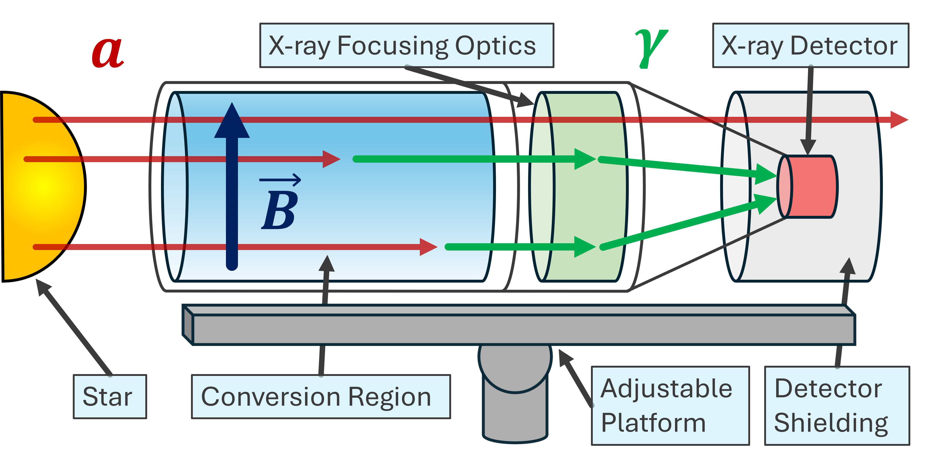
Figure 2.3: Conceptual diagram of a helioscope. Solar axions enter a magnetic conversion region mounted on a mobile platform that tracks the Sun. The converted X-ray photons are focused by X-ray optics onto a low-background detector.

The operating principle is illustrated in Figure 2.3. Solar axions traverse a strong transverse magnetic field and can convert into X-ray photons through the inverse Primakoff effect. Grazing-incidence optics focus those photons onto a detector optimized for the relevant energy range, while a mobile platform follows the Sun during the daily tracking window.

In natural units, $ℏ = 𝑐 = 1$ , the conversion probability for a homogeneous transverse magnetic field $𝐵_{⟂}$ of length $𝐿$ , neglecting photon absorption, is

𝑃_{𝑎 \to 𝛾} (𝐿) = {(\frac{𝑔_{𝑎 𝛾} 𝐵_{⟂} 𝐿}{2})}^{2} ℱ︀ (𝑞 𝐿) .

(2.1)

The coherence factor is

ℱ︀ (𝑞 𝐿) = {(\frac{2}{𝑞 𝐿})}^{2} {sin}^{2} (\frac{𝑞 𝐿}{2}) .

(2.2)

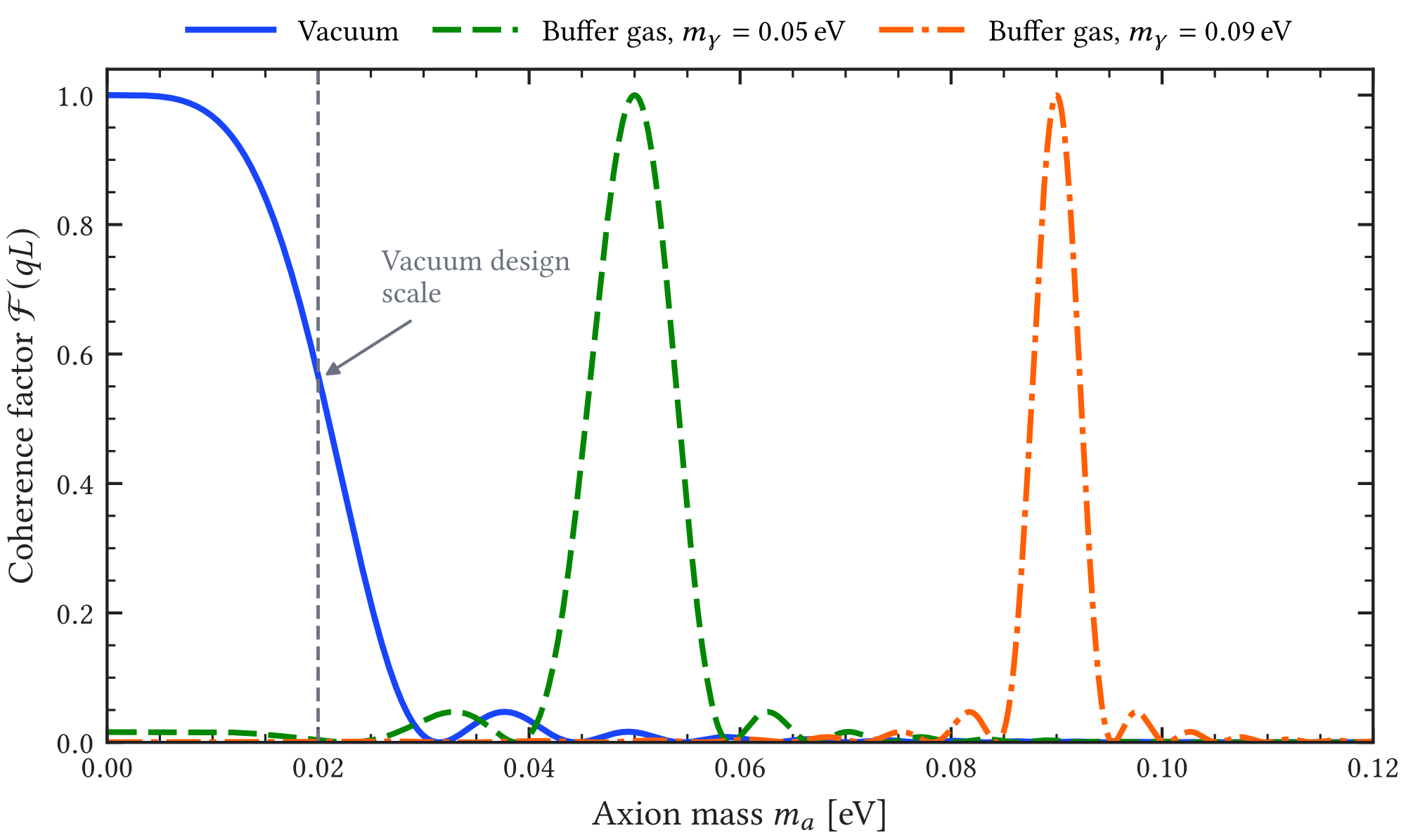
In vacuum, $𝑞 ≃ 𝑚_{𝑎}^{2} / (2 𝐸)$ for a relativistic axion of energy $𝐸$ . The coherent regime corresponds to $𝑞 𝐿 ≪ 1$ , for which $ℱ︀ ≃ 1$ and the conversion probability grows as $𝐵_{⟂}^{2} 𝐿^{2}$ .

At larger axion masses, the axion–photon momentum mismatch suppresses conversion. A buffer gas gives the photon an effective mass $𝑚_{𝛾}$ , changing the mismatch to $𝑞 ≃ | 𝑚_{𝑎}^{2} - 𝑚_{𝛾}^{2} | / (2 𝐸)$ and restoring coherence over a narrow mass interval. Equation (2.1) and Equation (2.2) remain the negligible-absorption expression after this substitution; a realistic gas scan must also include photon absorption and density gradients [49–51]. Vacuum is recovered by setting $𝑚_{𝛾} = 0$ .

For X-ray energies well above the atomic resonances of a low- $𝑍$ gas, the effective mass is its plasma frequency,

𝑚_{𝛾}^{2} = 𝜔_{pl}^{2} = \frac{4 𝜋 𝛼 𝑛_{𝑒}}{𝑚_{𝑒}} .

(2.3)

Here, $𝑛_{𝑒}$ is the electron density and $𝑚_{𝑒}$ is the electron mass. At fixed temperature and composition, $𝑛_{𝑒}$ is proportional to the gas pressure, so each pressure setting selects a different resonant value $𝑚_{𝑎} ≃ 𝑚_{𝛾}$ . The coherent interval at one setting is narrow; an extended mass range is therefore covered by increasing the pressure in overlapping steps rather than by operating at one fixed pressure. This relation between gas density, effective photon mass, and coherence is the basis of the CAST buffer-gas campaigns described below.

Figure 2.4: Coherence factor for 𝐸 = 4 keV axions in a 𝐿 = 10 m homogeneous magnetic field. Vacuum conversion remains coherent only at sufficiently low mass, whereas a buffer gas restores coherence around the mass for which 𝑚 𝑎 ≃ 𝑚 𝛾 . The illustrative gas curves neglect photon absorption and density gradients. — Figure 2.4: Coherence factor for $𝐸 = 4 keV$ axions in a $𝐿 = 10 m$ homogeneous magnetic field. Vacuum conversion remains coherent only at sufficiently low mass, whereas a buffer gas restores coherence around the mass for which $𝑚_{𝑎} ≃ 𝑚_{𝛾}$ . The illustrative gas curves neglect photon absorption and density gradients.

For one detection line, the expected differential event yield can be written schematically as

\frac{d 𝑁_{𝛾}}{d 𝐸} = \frac{d Φ_{𝑎}}{d 𝐸} 𝑃_{𝑎 \to 𝛾} (𝐸) 𝐴 𝜖_{𝑜} (𝐸) 𝜖_{𝑑} (𝐸) 𝜖_{𝑡} 𝑡 .

(2.4)

Here, $𝐴$ is the instrumented aperture, $𝜖_{𝑜}$ and $𝜖_{𝑑}$ are the optics and detector efficiencies, $𝜖_{𝑡}$ is the tracking fraction, and $𝑡$ is the elapsed data-taking time. For a selected focal region, $𝜖_{𝑜}$ includes the fraction of the solar image retained within it. For multiple detection lines, the predicted spectra are summed with their line-specific fields, apertures, and efficiencies. This expression connects the solar spectra and conversion probability to the experimental sensitivity parameters discussed next.

2.1.3 Experimental Figure of Merit

In the background-dominated regime, the principal design dependencies are summarized by the helioscope figure of merit (FOM) [13, 46]:

𝑓 = 𝑓_{𝑀} 𝑓_{𝐷 𝑂} 𝑓_{𝑇} .

(2.5)

Its components are

𝑓_{𝑀} = 𝐵_{eff}^{2} 𝐿^{2} 𝐴, 𝑓_{𝐷 𝑂} = \frac{𝜖_{𝑑} 𝜖_{𝑜}}{\sqrt{𝑏 𝑎}}, 𝑓_{𝑇} = \sqrt{𝜖_{𝑡} 𝑡} .

(2.6)

Here $𝐴$ is the total instrumented aperture and $𝐵_{eff}$ is the corresponding aperture-weighted effective transverse field; for a uniform field, $𝐵_{eff} = 𝐵_{⟂}$ . For a nonuniform magnet, $𝐵_{eff}^{2} 𝐿^{2} 𝐴$ denotes the field integral $\int_{𝐴} | \int_{0}^{𝐿} 𝐁_{⟂} d ℓ |^{2} d 𝐴$ in the coherent limit. The detector–optics term contains the detector efficiency $𝜖_{𝑑}$ , optics throughput $𝜖_{𝑜}$ , areal detector background level $𝑏$ , and selected focal-region area $𝑎$ . The latter includes the optics point-spread function and the finite angular extent of the solar source. The tracking term contains the tracking fraction $𝜖_{𝑡}$ and total elapsed time $𝑡$ .

This decomposition shows why a next-generation helioscope requires more than a strong magnet. The magnetic term increases with aperture, field strength, and length; the detector–optics term increases with efficiency and decreases with the selected area and background level; and the tracking term favors long daily exposure. Because the Primakoff signal scales as $𝑔_{𝑎 𝛾}^{4}$ , the projected coupling reach scales approximately as $| 𝑔_{𝑎 𝛾} | \propto 𝑓^{- 1 / 4}$ .

2.1.4 Sensitivity with Few Background Events

The figure of merit assumes coherent conversion and enough background counts for a Gaussian approximation; its original derivation uses approximately ten or more expected background events as a guide [46]. The lowest IAXO background targets can fall below this regime. For uniform background in an energy interval $Δ 𝐸$ and total focal area $𝑎$ ,

𝜇_{𝑏} = 𝑏 𝑎 Δ 𝐸 𝑇, 𝑇 = 𝜖_{𝑡} 𝑡,

(2.7)

where $𝑇$ is the effective tracking exposure. Combining the full-IAXO targets in Table 2.1 with an illustrative $2 – 7 keV$ window and $3 yr$ of elapsed operation gives $𝜇_{𝑏} = 2.84$ for $𝜖_{𝑡} = 0.5$ . If three years instead denotes effective tracking exposure, the expectation is $5.68$ events. These are alternative exposure definitions, not an uncertainty interval. The three-year run duration is drawn from the conceptual-design study [14]; the calculation does not reproduce its spectral acceptance or gas-scan exposure allocation.

For a Primakoff search at a fixed trial axion mass, a suitable starting point is the Poisson likelihood

ℒ︀ (𝑔_{𝑎 𝛾}, 𝝂) = \prod_{ℓ, 𝑘} Pois [𝑛_{ℓ 𝑘} | {(\frac{𝑔_{𝑎 𝛾}}{𝑔_{0}})}^{4} 𝑆_{ℓ 𝑘} (𝝂) + 𝐵_{ℓ 𝑘} (𝝂)] {ℒ︀}_{aux} (𝝂) .

(2.8)

Here $ℓ$ identifies a detection line and observing condition, including the gas density, and $𝑘$ identifies a bin in reconstructed energy and focal position. The signal $𝑆_{ℓ 𝑘}$ at a reference coupling $𝑔_{0}$ is obtained by folding the solar flux and magnetic conversion probability with the line-specific optics and detector response. The background expectation is $𝐵_{ℓ 𝑘}$ ; ${ℒ︀}_{aux}$ represents off-Sun measurements, calibrations, and finite-simulation constraints on nuisance parameters $𝝂$ . This construction preserves energy migration, focal containment, and selection losses instead of compressing them into one constant efficiency.

Figure 2.5 isolates the statistical effect using a single counting region with a known background mean $𝜇_{𝑏}$ . For a signal mean $𝑠 \geq 0$ , a prior uniform in $𝑠$ , and $𝑛$ observed events, the 95% Bayesian upper bound satisfies

\frac{\int_{0}^{𝑠_{95}} (𝑠 + 𝜇_{𝑏})^{𝑛} 𝑒^{- (𝑠 + 𝜇_{𝑏})} d 𝑠}{\int_{0}^{\infty} (𝑠 + 𝜇_{𝑏})^{𝑛} 𝑒^{- (𝑠 + 𝜇_{𝑏})} d 𝑠} = 0.95 .

(2.9)

The prior is uniform in $𝑔_{𝑎 𝛾}^{4}$ for a fixed Primakoff response, as in the CAST analysis [40]; other interval constructions need not give identical bounds [52]. At zero observed events, $𝑠_{95} = - ln (0.05) = 3.00$ . Expected sensitivity is evaluated over $𝑛 \sim Pois (𝜇_{𝑏})$ , rather than by setting an observed count equal to a possibly noninteger mean. For the illustrative $𝜇_{𝑏} = 2.84$ and $5.68$ , the median background-only outcomes are three and six events, respectively. Their signal upper bounds are $𝑠_{95} = 5.48$ and $6.91$ , corresponding to coupling limits approximately 16% and 23% above the zero-background value at fixed signal response and exposure.

Figure 2.5: Relative 95% coupling upper limit for the single-region model in Equation (2.9) , holding exposure and signal response fixed. The solid curve is the median over background-only Poisson outcomes, divided by the zero-background limit; the shaded region contains the central 68.27% quantiles of those outcomes and is not a parameter-confidence interval. Discontinuities arise from the discrete event count. The dashed curve gives the large-background approximation for the same prior. Background normalization is treated as known in this illustration; no absolute BabyIAXO coupling reach is inferred. — Figure 2.5: Relative 95% coupling upper limit for the single-region model in Equation (2.9), holding exposure and signal response fixed. The solid curve is the median over background-only Poisson outcomes, divided by the zero-background limit; the shaded region contains the central 68.27% quantiles of those outcomes and is not a parameter-confidence interval. Discontinuities arise from the discrete event count. The dashed curve gives the large-background approximation for the same prior. Background normalization is treated as known in this illustration; no absolute BabyIAXO coupling reach is inferred.

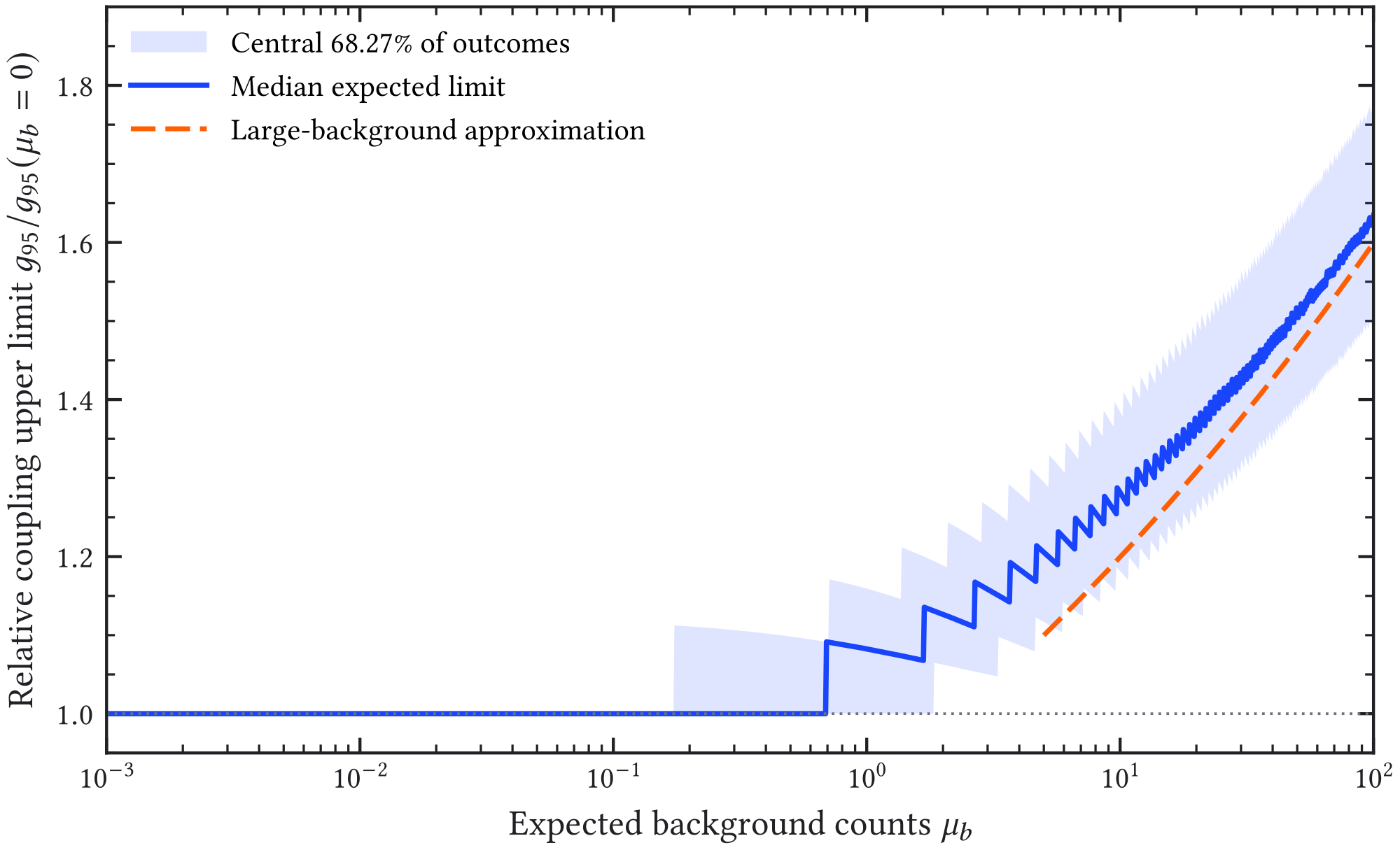
The background-dominated scaling is $𝑔_{𝑎 𝛾}^{lim} \propto 𝑏^{1 / 8} 𝑇^{- 1 / 8}$ when the spectrum and efficiencies are fixed. Once the median outcome is zero, further background reduction leaves the counting limit approximately unchanged, while increasing the accepted signal exposure gives $𝑔_{𝑎 𝛾}^{lim} \propto 𝑇^{- 1 / 4}$ . A veto or topology requirement should therefore be optimized through its effect on both the signal acceptance and the Poisson limit. The literature projections below retain their original assumptions; the detector studies in this thesis do not supply all inputs required to replace them with an absolute BabyIAXO prediction.

2.2 From CAST to IAXO

2.2.1 CAST as the Reference Helioscope

The CERN Axion Solar Telescope (CAST) established the reference implementation of the modern helioscope technique [12]. It used a repurposed Large Hadron Collider (LHC) test dipole magnet with two parallel bores, instrumented at both ends by several low-background X-ray detector systems. From 2002 to 2006, the sunset end used a conventional TPC covering both bores, while the sunrise end combined a Micromegas detector on one bore with a pn-CCD behind an X-ray telescope on the other [53–55]. The optics reduced the detector area over which signal events were sought, demonstrating directly the background-count advantage later formalized in the detector–optics term of the helioscope figure of merit. After aging degraded the TPC, the sunset system and the original sunrise Micromegas were replaced by a new generation of shielded Micromegas detectors. Microbulk fabrication, improved radiopurity, refined event-topology discrimination, and progressively more complete passive and active shielding then reduced their background level. In 2014, a purpose-built slumped-glass telescope was coupled to a Micromegas detector, forming the IAXO pathfinder and demonstrating the combined optics, shielding, veto, and readout concept adopted for the next-generation program [40, 56].

CAST separated the mass scan into three principal operating regimes, summarized in Figure 2.6. The evacuated-bore phase retained coherence for $𝑚_{𝑎} ≲ 0.02 eV$ . The first buffer-gas campaign used $^{4} He$ at $1.8 K$ : 160 density settings, equivalent to pressure increments of approximately $0.08 mbar$ and reaching $13.4 mbar$ , covered $0.02 – 0.39 eV$ . The lower saturated-vapor pressure of $^{4} He$ limited the accessible density. Replacing it with $^{3} He$ allowed higher pressures at the same magnet temperature; successive scans covered $0.39 – 1.17 eV$ , with the pressure chosen so neighboring coherence windows overlapped [49–51].

Figure 2.6: Axion-mass coverage of the principal CAST operating regimes. The vacuum interval is set by loss of coherence in the 9.26 m magnet. The 4 He and 3 He intervals were scanned through many overlapping density settings; each individual setting was resonant only over a narrow mass interval. End points summarize the published campaign ranges and should not be interpreted as identical coupling sensitivity throughout each interval [ 49 – 51 ]. — Figure 2.6: Axion-mass coverage of the principal CAST operating regimes. The vacuum interval is set by loss of coherence in the $9.26 m$ magnet. The $^{4} He$ and $^{3} He$ intervals were scanned through many overlapping density settings; each individual setting was resonant only over a narrow mass interval. End points summarize the published campaign ranges and should not be interpreted as identical coupling sensitivity throughout each interval [49–51].

CAST demonstrated low detector-background levels under helioscope conditions, the background-count reduction obtained by focusing, and reliable long-term operation of a Sun-tracking magnet and its detection lines. Its extended run with the IAXO pathfinder and a xenon-based Micromegas detector found no axion signal and set $| 𝑔_{𝑎 𝛾} | < 5.8 \times 10^{- 11} {GeV}^{- 1}$ at 95% confidence for $𝑚_{𝑎} ≲ 0.02 eV$ [40]. This result links the strongest demonstrated helioscope limit to the detector family, focusing concept, and background-control methods developed further for the BabyIAXO stage.

2.2.2 Why a Dedicated Helioscope Is Required

CAST also exposed the limitations of a repurposed accelerator magnet: small total aperture, constrained detector and optics geometry, and limited tracking time. Because the figure of merit depends on both the magnetic aperture and the detector–optics term, a substantial sensitivity improvement requires a dedicated experimental design rather than incremental upgrades to an existing accelerator component.

Parameter	CAST	BabyIAXO	IAXO
Magnet concept	repurposed LHC dipole	purpose-built dipole	purpose-built toroid
Representative field $𝐵$ [ $T$ ]	$9$	$\sim 2$	$\sim 2.5$
Magnetic length $𝐿$ [ $m$ ]	$9.26$	$\sim 10$	$\sim 20$
Total aperture $𝐴$ [ $m^{2}$ ]	$\sim 0.003$	$\sim 0.77$	$\sim 2.3$
Magnet FOM $𝑓_{𝑀}$ [ $T^{2} m^{4}$ ]	$\sim 21$	$\sim 230$	$\sim 6000$
Background level $𝑏$	$\sim 10^{- 6}$	$\sim 10^{- 7}$	$\sim 10^{- 8}$
Focal-region area $𝑎$ [ ${cm}^{2}$ ]	$0.15$	$2 \times 0.3$	$8 \times 0.15$
Tracking fraction $𝜖_{𝑡}$	$\sim 0.12$	$\sim 0.5$	$\sim 0.5$

Table 2.1: Published conceptual-design sensitivity benchmarks for CAST, BabyIAXO, and IAXO [12–14]. The aperture

𝐴

is the total over the instrumented bores, and the entries for

𝑎

state the number of detection lines times the representative area per line. The background level

𝑏

is given in

counts {keV}^{- 1} {cm}^{- 2} s^{- 1}

. The quoted

𝑓_{𝑀}

values come from detailed magnetic-field models and therefore need not equal the result obtained from the rounded values of

𝐵

𝐿

, and

𝐴

shown in the table. The CAST detector parameters represent the IAXO-pathfinder configuration rather than every detector used during CAST.

Table 2.1 summarizes the resulting design shift. CAST exploited the high field of an accelerator dipole, whereas BabyIAXO and IAXO exchange some field strength for much larger aperture, systematic use of focusing optics, lower detector-background targets, and substantially longer solar tracking. The IAXO strategy is therefore to co-optimize $𝑓_{𝑀}$ , $𝑓_{𝐷 𝑂}$ , and $𝑓_{𝑇}$ in a purpose-built instrument [13, 46, 57].

2.3 The IAXO Experiment

2.3.1 Physics Reach and Design Philosophy

IAXO is conceived as a next-generation axion helioscope optimized for solar axions and ALPs [13, 45, 57]. In the low-mass region, design projections improve the background-limited signal-to-noise ratio relative to CAST by approximately four to five orders of magnitude. They correspond to a projected sensitivity near $| 𝑔_{𝑎 𝛾} | \sim 3 \times 10^{- 12} {GeV}^{- 1}$ , approximately a factor of 20 below the current CAST limit, subject to the assumed exposure and background performance [45]. The observatory is also designed to probe solar production through $𝑔_{𝑎 𝑒}$ with sensitivity beyond previous laboratory searches.

Figure 2.7: Helioscope-relevant axion–photon parameter space. The CAST and stellar-cooling bounds and the BabyIAXO/IAXO projection curves are redrawn from checksum-verified data in the AxionLimits snapshot pinned to Git commit 7d375f4 [ 39 ]. The original CAST and globular-cluster results are given in Refs. [ 40 , 41 ], and the conceptual-design projections in Refs. [ 14 , 58 ]. Solid boundaries with shading denote observed exclusions, whereas unfilled dashed or dotted curves denote heterogeneous design projections. The hatched QCD-axion band uses the central mass–coupling constants in Eqs. Equation (2.4) and Equation (2.5) and is not an exclusion [ 8 ]. Within it, the solid and dashed brown lines mark the KSVZ ( 𝐸 / 𝑁 = 0 ) and DFSZ ( 𝐸 / 𝑁 = 8 / 3 ) benchmark relations, respectively. IAXO+ denotes the optimistic ultimate reach of the IAXO research-and-development program, not a separately approved experimental stage [ 58 ]. — Figure 2.7: Helioscope-relevant axion–photon parameter space. The CAST and stellar-cooling bounds and the BabyIAXO/IAXO projection curves are redrawn from checksum-verified data in the AxionLimits snapshot pinned to Git commit `7d375f4` [39]. The original CAST and globular-cluster results are given in Refs. [40, 41], and the conceptual-design projections in Refs. [14, 58]. Solid boundaries with shading denote observed exclusions, whereas unfilled dashed or dotted curves denote heterogeneous design projections. The hatched QCD-axion band uses the central mass–coupling constants in Eqs. Equation (2.4) and Equation (2.5) and is not an exclusion [8]. Within it, the solid and dashed brown lines mark the KSVZ ( $𝐸 / 𝑁 = 0$ ) and DFSZ ( $𝐸 / 𝑁 = 8 / 3$ ) benchmark relations, respectively. IAXO+ denotes the optimistic ultimate reach of the IAXO research-and-development program, not a separately approved experimental stage [58].

These projections set the performance targets for the coupled subsystems discussed below: magnetic conversion aperture, X-ray optics and focal-plane background, and solar-tracking exposure. The IAXO+ curve is retained only as an optimistic performance benchmark; the baseline experimental stages discussed in this thesis are BabyIAXO and IAXO. The projection curves reproduce heterogeneous literature assumptions and were not recalculated from the March 2026 engineering parameters. Observed boundaries are digitized approximations; the current published CAST plateau is the $5.8 \times 10^{- 11} {GeV}^{- 1}$ limit quoted above.

2.3.2 Magnet

The 2014 reference design for IAXO uses a superconducting toroidal magnet approximately $20 m$ long, formed by eight coils and providing eight bores of approximately $60 cm$ diameter [13]. The useful field in the bores is approximately $2.5 T$ , while the peak field in the windings is about $5.4 T$ ; the principal gain over CAST comes from the much larger integrated magnetic aperture. The toroidal layout leaves the bores accessible for optics and detectors and defines eight parallel detection lines. The bores can operate in vacuum or, for higher-mass scans, with a buffer gas.

The final magnet design remains part of the post-BabyIAXO program. Recent studies retain the large multi-bore concept while also considering high-temperature-superconductor alternatives that could change the field and cryogenic implementation [45].

2.3.3 X-ray Optics

The reference IAXO design equips every detection line with grazing-incidence X-ray optics [13, 59]. The sensitivity benchmark in Table 2.1 assumes a selected focal-region area of approximately $0.15 {cm}^{2}$ per line. Detailed designs optimize both the energy-dependent throughput and the focal image of the extended solar source.

Focusing does not reduce the areal detector background level $𝑏$ . Instead, it confines the signal to a small selected area $𝑎$ , reducing the expected background counts in the signal region in proportion to $𝑏 𝑎$ when the background is approximately uniform. This coupling between optics and detector performance is the origin of the detector–optics term in Equation (2.6).

2.3.4 Detector Technologies

The focal-plane detectors must combine high efficiency in the reference $1 – 10 keV$ band with stage-dependent background targets. The BabyIAXO sensitivity benchmark assumes a background level of $1 \times 10^{- 7} counts {keV}^{- 1} {cm}^{- 2} s^{- 1}$ , whereas the full IAXO concept targets $1 \times 10^{- 8} counts {keV}^{- 1} {cm}^{- 2} s^{- 1}$ [13, 14]. Under the surface conditions considered for the program, meeting these targets requires radiopure construction, passive shielding, topology-based discrimination, and active-veto systems [17].

Microbulk Micromegas detectors are the most developed gaseous technology for this role because CAST and IAXO-D0 demonstrated their radiopurity, topological discrimination, stable operation, and compatibility with focused soft X rays. Alternative focal-plane concepts include GridPix detectors, metallic magnetic calorimeters, transition-edge sensors, and silicon drift detectors; their lower thresholds or improved energy resolution are particularly relevant to the softer ABC spectrum [45, 60, 61]. Section 3 develops the Micromegas detector line used in this thesis.

2.3.5 Tracking and Observatory Operation

The reference IAXO concept mounts the magnet, optics, and detectors on elevation and azimuth drives that provide solar tracking for up to approximately half of each day, corresponding to $𝜖_{𝑡} ≃ 0.5$ [13]. The moving structure must support the cold mass, preserve alignment among the bores, optics, and detectors, and allow reproducible transitions between Sun-tracking data and off-Sun background measurements. These requirements enter both the sensitivity exposure and the background-control strategy.

The conceptual installations are surface facilities rather than deep-underground laboratories. Background suppression must therefore be obtained through the detector, passive shielding, event-topology analysis, and active vetoing. The evolution of the specific BabyIAXO site assumption, and its consequences for this thesis, are discussed below.

2.4 BabyIAXO as an Intermediate Stage

2.4.1 Role Within the IAXO Program

BabyIAXO is the intermediate experimental stage between CAST and the full IAXO observatory [14, 45, 58]. It provides a common environment in which the magnet, optics, detectors, cryogenics, tracking, alignment, gas handling, and data acquisition can be integrated and commissioned. At the same time, it is a physics instrument with independent discovery reach. This staged program also builds the shared analysis, software, operations, and system-integration experience required for the full observatory.

Under the 2021 conceptual-design assumptions, including $1.5 yr$ of effective exposure for each of the vacuum and buffer-gas campaigns, the projected low-mass vacuum sensitivity is $| 𝑔_{𝑎 𝛾} | ≃ 1.5 \times 10^{- 11} {GeV}^{- 1}$ for $𝑚_{𝑎} ≲ 0.02 eV$ . The projected buffer-gas scan would extend the reach to higher masses and probe the KSVZ benchmark approximately over $0.06 – 0.25 eV$ [14]. BabyIAXO therefore combines new physics reach with validation of the technologies and subsystem interfaces required for the full observatory.

Figure 2.8: Annotated view of the current BabyIAXO integration model, adapted from the March 2026 superconducting-dipole status presentation [ 62 ]. The rendering identifies the superconducting dipole, one optics–detector line, and the azimuth–elevation support used for solar tracking. — Figure 2.8: Annotated view of the current BabyIAXO integration model, adapted from the March 2026 superconducting-dipole status presentation [62]. The rendering identifies the superconducting dipole, one optics–detector line, and the azimuth–elevation support used for solar tracking.

2.4.2 Main Experimental Features

The 2021 conceptual design established a common-coil dipole with two parallel flat racetrack coils carrying opposite currents and two $10 m$ -class bores [14]. By March 2026, the engineering model specified two $11 m$ -long free bores of $0.70 m$ diameter and an aluminum-stabilized NbTi/Cu Rutherford-cable conductor operated at $6 kA$ [62]. At that operating current, the calculated mean transverse bore field is $2.1 T$ , the peak field on the cable is $4.7 T$ , and the three-dimensional magnet figure of merit is approximately $290 T^{2} m^{4}$ . The public June 2026 status presentation retained these engineering values [63]. Each bore can host a complete detection line with dimensions representative of the full observatory, allowing the magnet aperture, cryogenic integration, and detector interfaces to be tested at full line scale before the final toroidal observatory is designed.

Figure 2.9: Three-dimensional magnetic-field model of the current BabyIAXO common-coil dipole, adapted from the March 2026 superconducting-dipole status presentation [ 62 ]. Color encodes the field magnitude | 𝐁 | in tesla, and the inset provides a transverse field-map detail through the straight coil sections. The peak field occurs in the conductor and must not be confused with the 2.1 T mean transverse field in the two 0.70 m -diameter free bores. — Figure 2.9: Three-dimensional magnetic-field model of the current BabyIAXO common-coil dipole, adapted from the March 2026 superconducting-dipole status presentation [62]. Color encodes the field magnitude $| 𝐁 |$ in tesla, and the inset provides a transverse field-map detail through the straight coil sections. The peak field occurs in the conductor and must not be confused with the $2.1 T$ mean transverse field in the two $0.70 m$ -diameter free bores.

On August 11, 2026, the University of Bonn announced approval of a magnet system costing EUR 6 million, financed by EUR 3 million from the German Research Foundation (DFG), EUR 2.4 million from North Rhine-Westphalia, and EUR 0.6 million from the participating universities [64]. This funding milestone concerns magnet construction; it does not establish completion of the magnet or approval of the final DESY site.

The 2021 conceptual optics baseline paired one custom, NuSTAR-derived segmented-glass telescope with an available XMM-Newton flight-spare telescope [14]. By the 23rd IAXO Collaboration Meeting in March 2026, the optics program also included BRAVO-SUN and XRISM-derived components and was developing a co-mounted telescope configuration. The final combination of components remained under development [65]. The June 2026 public comparison quoted approximately $0.2 {cm}^{2}$ for the custom telescope and $0.3 – 0.7 {cm}^{2}$ for the XMM telescope [63]. These areas cannot be applied interchangeably: each line requires its own energy-dependent throughput and focal containment, evaluated for the chosen signal region.

Micromegas remain the principal low-background technology for the detector line studied here, while the broader BabyIAXO program also develops GridPix and cryogenic focal-plane detectors [14, 61]. The detector line treated in this thesis is therefore one implementation within a broader focal-plane program.

2.4.3 Evolution of the DESY Site Scenario

When the background-model and veto-simulation program began, the reference BabyIAXO site was the HERA South Hall on the DESY campus. The hall is an underground accelerator space rather than a deep-underground low-background laboratory, but its structure, access shafts, and surrounding material could modify the cosmic-ray field relative to an outdoor installation. Early simulations therefore treated the cosmic-ray component as site dependent, with attention to overburden, openings, and local shielding.

Figure 2.10: Adapted comparison of the HERA South Hall context with the on-surface BabyIAXO working scenario presented at the 23rd IAXO Collaboration Meeting in March 2026 [ 66 ]. The underlying DESY campus aerial photograph retains its © DESY credit. The on-surface option removes any assumed hall overburden from the environmental boundary conditions used for detector-background studies. — Figure 2.10: Adapted comparison of the HERA South Hall context with the on-surface BabyIAXO working scenario presented at the 23rd IAXO Collaboration Meeting in March 2026 [66]. The underlying DESY campus aerial photograph retains its © DESY credit. The on-surface option removes any assumed hall overburden from the environmental boundary conditions used for detector-background studies.

During 2025 and 2026, internal collaboration studies shifted the working baseline toward an outdoor, on-surface location on the DESY campus. The reported considerations included simpler civil infrastructure, reduced demands on DESY infrastructure resources, lower expected cost, and a shorter route to site activation [67]. As reported at the 23rd collaboration meeting in March 2026, the DESY directorate had encouraged further site exploration and development of cost and schedule plans. This did not constitute formal project or site approval, and the exact position and site elevation remained under study [15].

The March 2026 on-surface working baseline is adopted here without credit for hall overburden. Simulations that retain boundary conditions associated with HERA South are identified separately. An outdoor source spectrum is not a demonstrated upper bound on every local contribution: the ground, housing, platform, and magnet can attenuate primaries while generating or redistributing secondaries. Transfer to the final site therefore requires a consistently normalized source boundary and transport through the local environment. The detector system must address sea-level muons, neutrons, and secondary particle production in the passive shielding. An active veto is therefore central to the mitigation strategy investigated here; Section 5 evaluates the proposed plastic-scintillator veto with cadmium neutron-capture layers.

2.5 Connection to the Present Thesis

Section 3 narrows the discussion from the helioscope to the detector-development line. It introduces time-projection-chamber signal formation and microbulk Micromegas technology, then describes the IAXO-D0 experimental prototype and the IAXO-D1 simulation geometry used in this work. Section 4 develops the REST-for-Physics/restG4 framework used to represent that detector and its environment. Section 5 and Section 6 evaluate the active-veto strategy and assemble the validated components and remaining limitations of the partial background model.