Experimental Typst web edition · Veto chapter pilot
5 Shielding and Veto System
Introduction
The current BabyIAXO working baseline assumes an on-surface installation at DESY, where passive shielding must suppress environmental photons without the benefit of underground overburden. The same lead that provides this attenuation does not efficiently moderate fast neutrons and can convert them into secondary neutrons, photons, and charged fragments. The active shield must therefore perform two functions: reject through-going cosmic muons and tag the distributed prompt and post-trigger activity associated with neutron-induced showers.
This chapter presents the physical argument and experimental evidence that led to a three-stage scintillator–cadmium veto surrounding the lead shield. The narrative is organized around the design decisions: why passive shielding is insufficient, how the active stages sample the neutron-induced shower, why three layers were selected, how the waveform information is reduced to veto observables, and what the commissioned IAXO-D0 prototype demonstrates in data. Detailed nuclear-data benchmarks, campaign metadata, full diagnostic scans, and the technical construction of the late-window control analysis are retained in the Appendix.
The division of scope with Section 6 is explicit. This chapter addresses veto physics, conditional rejection, calibration-like control acceptance, and prototype validation, including the published IAXO-D0 data cut flow. Section 6 provides the source normalization, confidence intervals on source-normalized simulation levels, and prompt/delayed accounting used in the conservative partial source-response model. The common REST-for-Physics/restG4 implementation is described in the software [83–86].
5.1 Design boundary and source inputs
5.1.1 Detector configurations and requirements
Three related detector configurations appear in this chapter and should not be conflated. The optimization simulations use the 59-panel veto geometry developed for the detector line. The experimental validation uses the commissioned 57-panel IAXO-D0 surface prototype. A detector-and-site prediction for BabyIAXO at DESY can be made only after the corresponding contracts are frozen; it is not inferred by rescaling the Zaragoza prototype result.
| Configuration | Role in this chapter | Quantitative use |
|---|---|---|
| 59-panel simulated veto | Three scintillator–cadmium stages around the lead shield | Geometry and layer optimization; conditional waveform-level rejection |
| 57-panel IAXO-D0 prototype | Commissioned surface setup in Zaragoza | Published 52.1-day data cut flow and waveform-level validation |
| BabyIAXO projection at DESY | Planned detector and site configuration; not yet frozen | Requires site-specific source transfer, final channel map, and a separately validated response contract |
The design must preserve X-ray-like Micromegas events in the keV region while rejecting surface backgrounds. It must remain compatible with the X-ray beam path, services, mechanical clearances, available scintillator modules, and the synchronized AGET-based readout. The beam pipe prevents perfectly hermetic passive shielding, whereas the neutron-capture timescale requires a readout window long enough to retain post-trigger activity without accepting an excessive number of random coincidences. These constraints make geometry, timing, and analysis inseparable parts of the veto design.
5.1.2 Surface source inputs
The selected design studies use source-specific inputs rather than one generic “cosmic” sample. Production muons use the correlated sea-level parameterization of Guan et al. implemented by the CosmicMuons generator [104]. The neutron layer scans use the outdoor HENSA spectrum in the – interval [105, 106]. Their nominal input histogram is proportional to , but the inspected projected-source reader applies an additional factor, producing a sampled density proportional to . The input histogram and sampled angular law must therefore be distinguished when interpreting the layer and inclination scans. The campaign normalization and angular-measure audit are documented in Section 6; the geometry comparisons here retain their common historical source setting. Historical passive-shield scans and cross-checks use CRY, while EXPACS provides an independent spectral comparison [88, 107, 108].
The HENSA outdoor field includes atmospheric and environment-modified neutrons measured at the surface. It is therefore described below as the HENSA outdoor neutron field, not as a pure cosmic component. It must not be added to the HENSA-minus-CRY environmental residual as if the two were independent source terms. The generator implementation is documented in Section 4.6.5; the source normalization and non-additivity convention are defined in Section 6.5.1.4.
5.2 Limits of passive shielding
5.2.1 Material roles
Lead remains essential because it strongly attenuates environmental photons. Its role for fast neutrons is different. In an elastic collision with a nucleus of mass number , the maximum transferable fraction of neutron kinetic energy is , which is unity for hydrogen but only about for lead. Consequently, lead is a poor moderator, while inelastic and neutron-emission channels produce a secondary shower once the incident energy reaches the MeV range.
Hydrogen-rich plastic scintillator complements the lead by slowing secondary neutrons and converting recoil-proton and charged-particle energy into light. Cadmium is placed only after this moderation step: its large thermal-neutron capture probability converts the slowed component into a gamma cascade near an active panel. The nuclear de-excitation is prompt relative to the capture, but moderation can place the capture and its scintillator response well after the Micromegas trigger. The signal medium itself remains sensitive to compact secondary photons and electrons as well as to nuclear recoils, so the veto must tag the surrounding history rather than identify the primary particle from the Micromegas deposit alone.
The transport-model checks that support this mechanism are summarized in Section 5.3.3 and documented in Appendix Section A.2.
5.2.2 Lead thickness and penetrations
A parameterized lead-shield scan was performed with idealized coverage and with the X-ray beam-pipe opening. The historical CRY samples are used here only to compare geometries under a common source definition; they do not define the final absolute background level. The full per-particle results are retained in Appendix Section A.11.
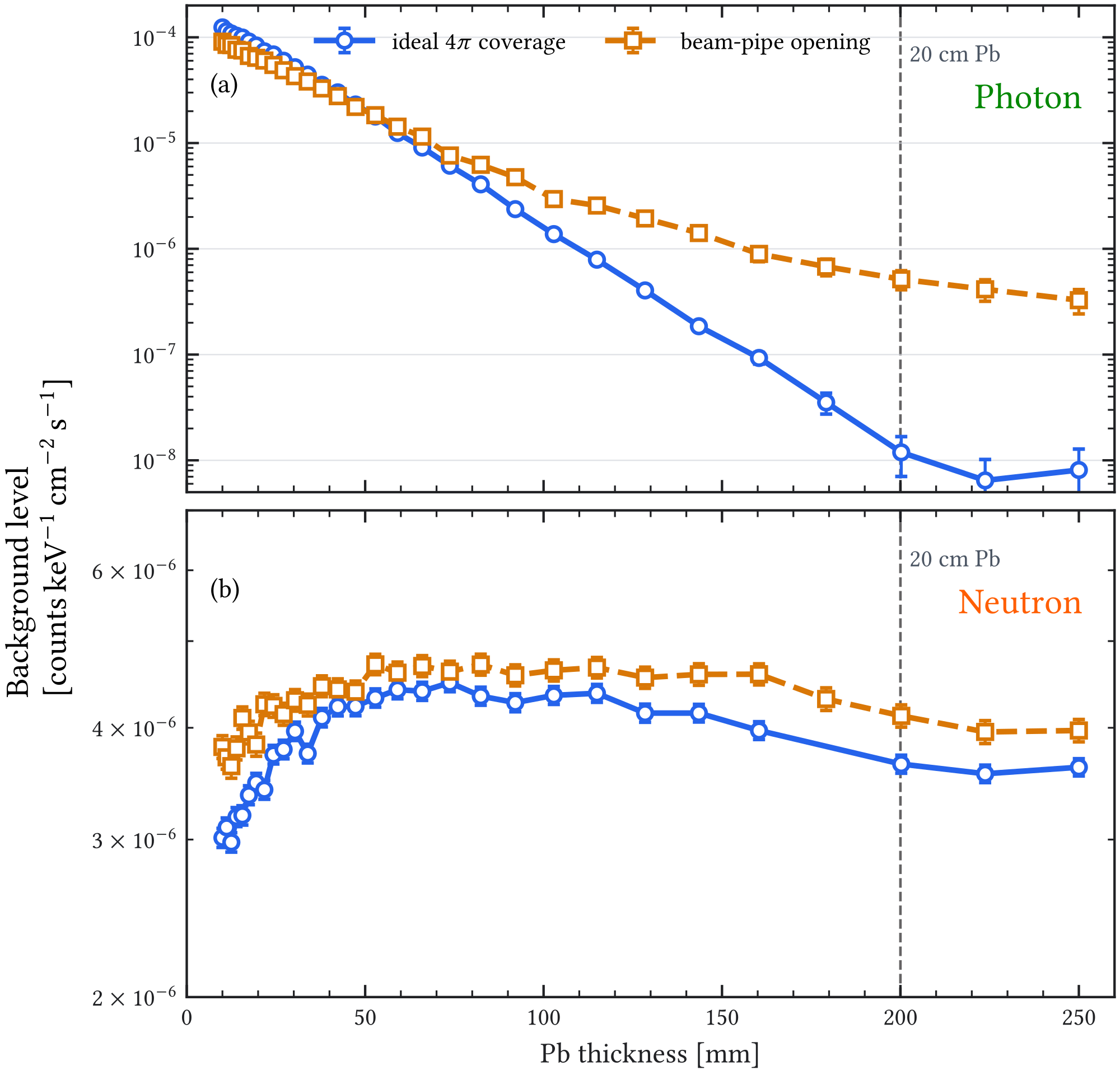
The photon response improves by more than four orders of magnitude over the idealized scan and by roughly a factor when the pipe opening is included. The neutron response remains within the same order of magnitude and exhibits a broad intermediate-thickness enhancement. The design consequence is robust: thick lead is retained for photon suppression, but increasing its thickness does not replace an active neutron-sensitive system.
5.2.3 Passive neutron moderation
Borated high-density polyethylene (HDPE) was tested as a moderator and absorber while retaining the total lead thickness required for photon attenuation [105]. The scan varied both the HDPE thickness and its position within a Pb/HDPE/Pb stack. Hydrogen slows the neutron population, and the dominant excited-state branch of releases a gamma after capture. The usefulness of this mechanism depends on where moderation and capture occur relative to the lead and the detector.
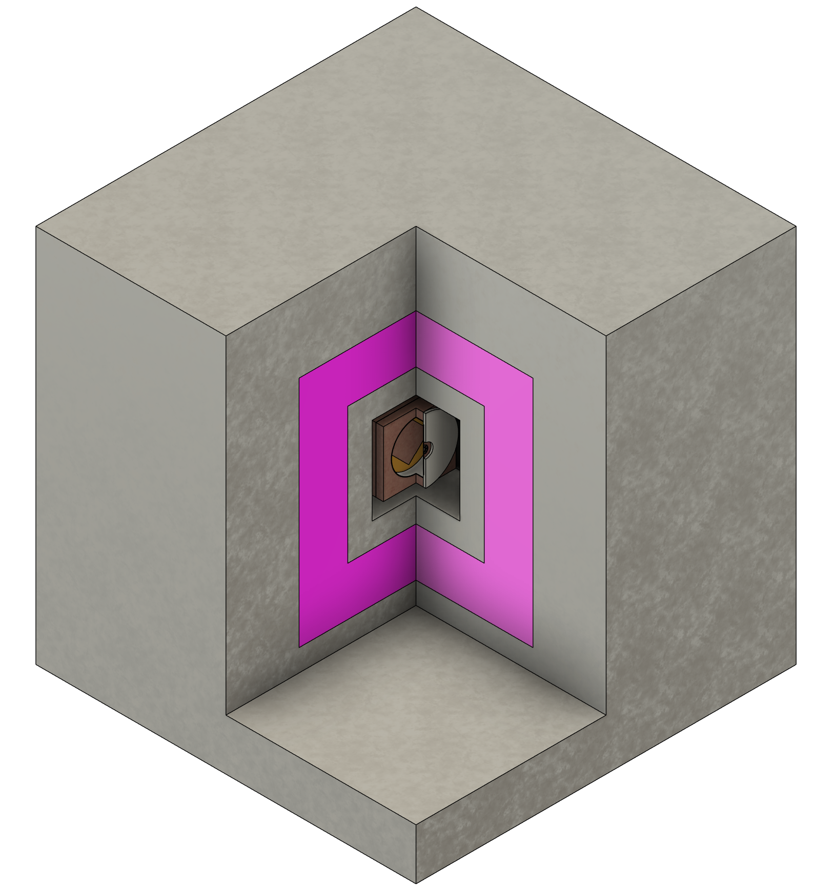
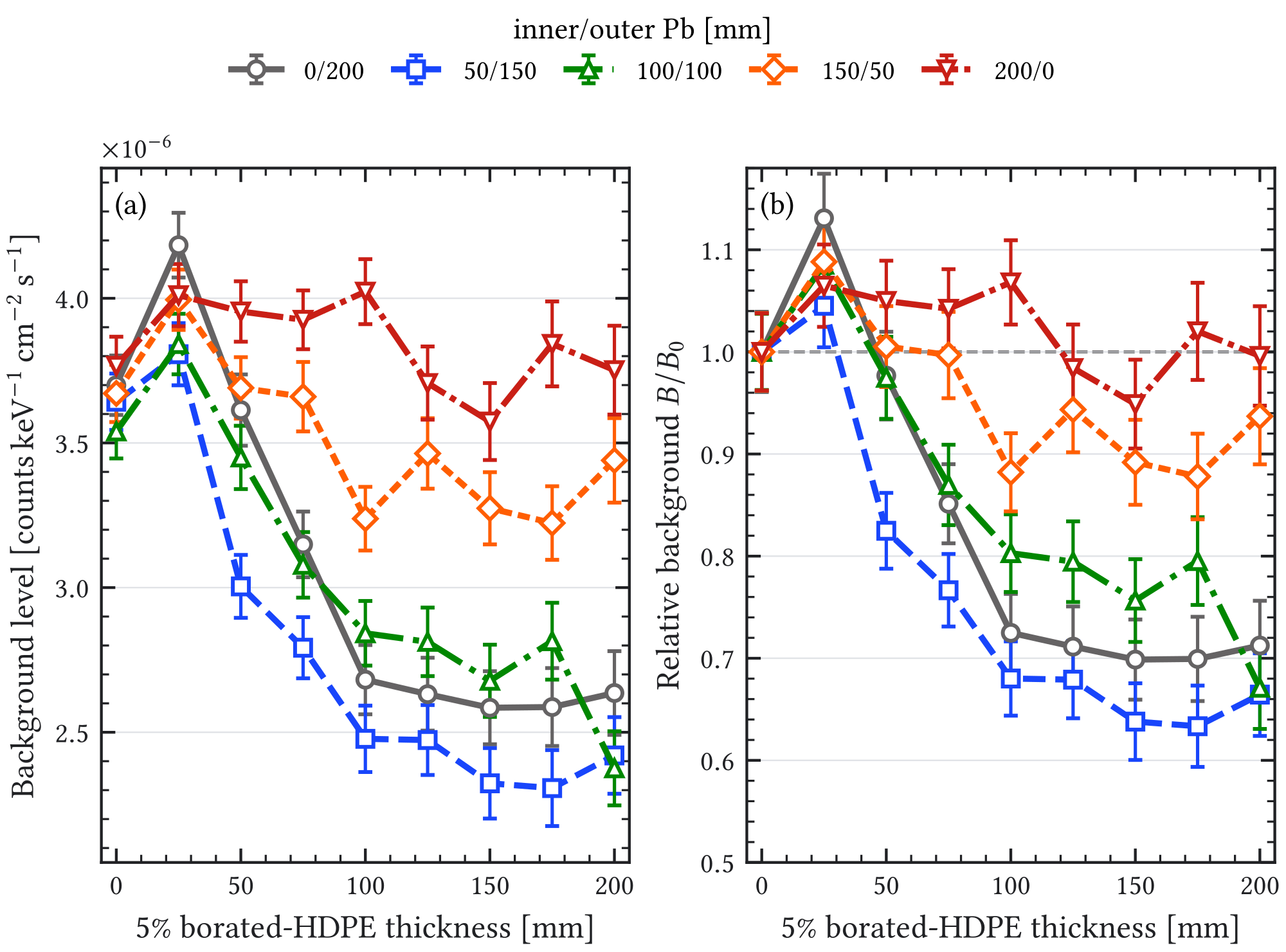
The most favorable configurations reduce the neutron response by only –, corresponding to a suppression factor of order . Practical moderator thicknesses do not thermalize the full MeV–GeV component before secondary production has occurred in the lead and surrounding structures. This result defines the active-veto boundary condition: the lead remains in place, and the active panels are arranged to sample the shower that it produces.
5.3 Neutron-sensitive active veto concept
5.3.1 From surface primaries to taggable secondaries
The integral surface-neutron field is not, by itself, the population that controls the detector response. Low-energy neutrons are abundant in the outdoor spectrum, but the primaries that produce Micromegas-sensitive activity after traversing the shielding are much harder. In the HENSA three-layer diagnostic, 59.68% of the detector-reaching population lies between and , and a further 31.78% lies between and . The historical CRY cross-check exhibits the same qualitative hardening. The comparison in Figure 5.3 is normalized within each source and detector-reaching sample; it establishes the relevant energy range but is not an absolute source comparison.
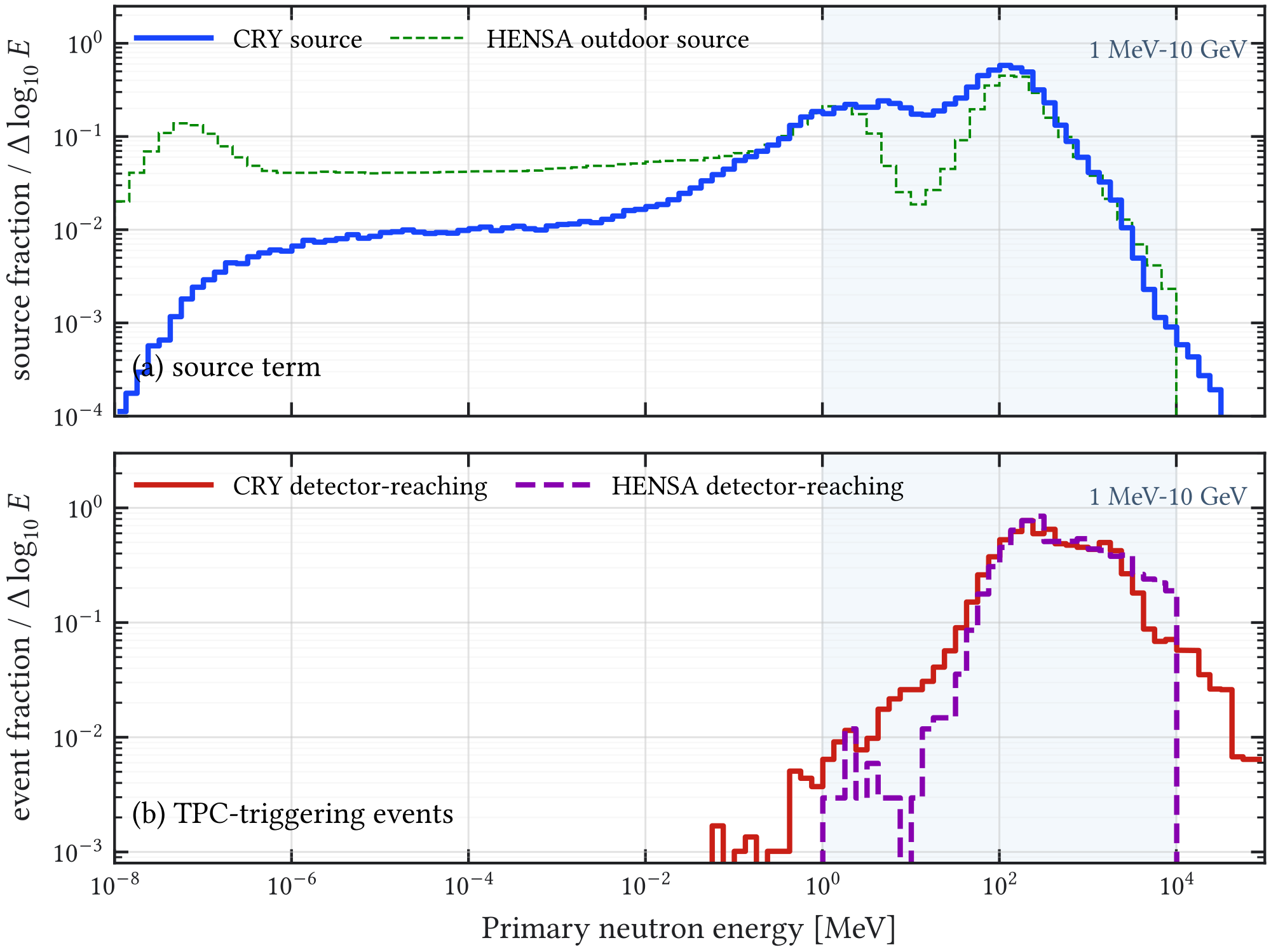
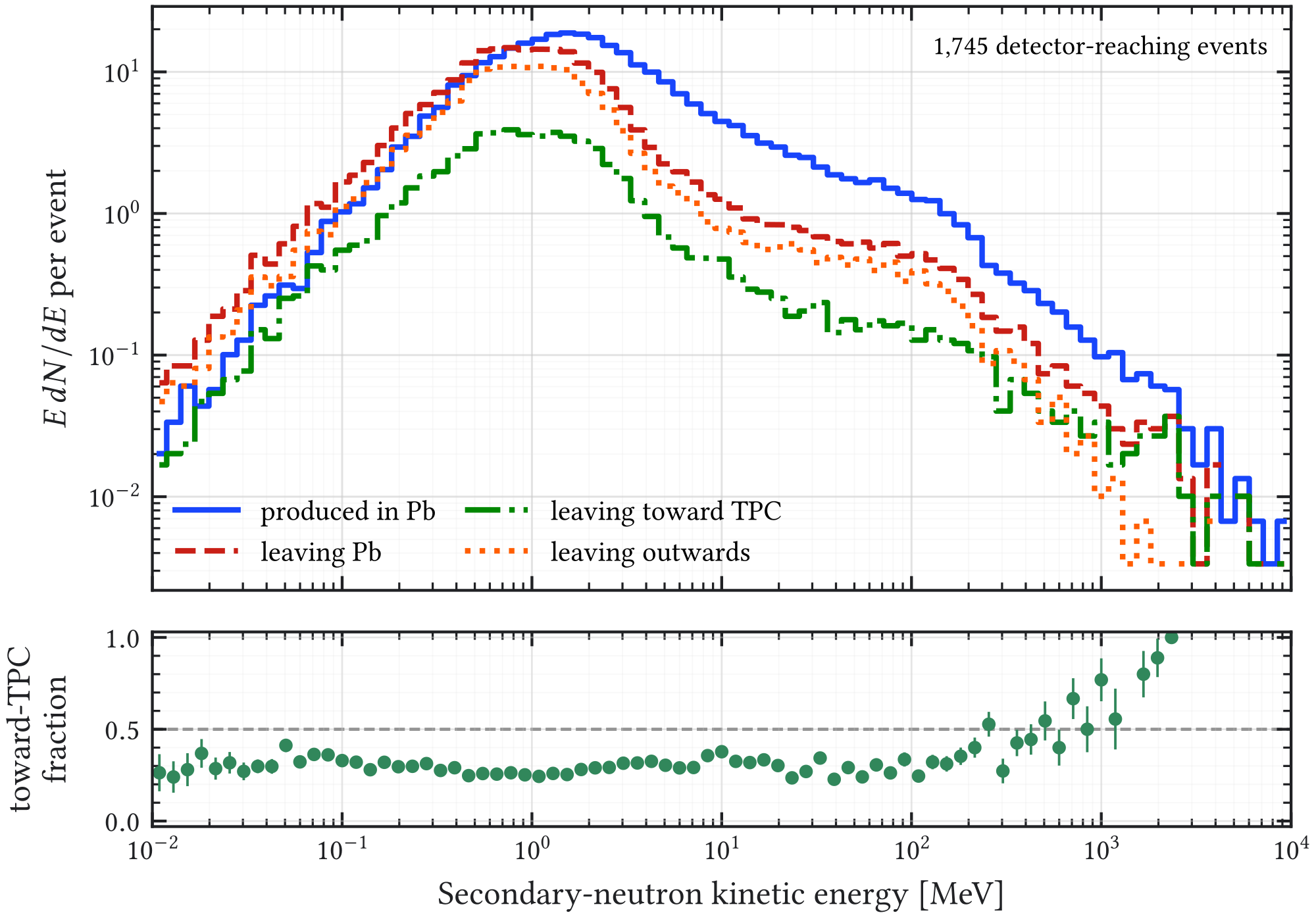
CRY and HENSA outdoor source shapes; the lower panel shows the corresponding detector-reaching populations. The HENSA production is restricted to –. The hardening demonstrates that the detector-relevant population is selected from the high-energy tail rather than from the dominant low-energy source fluence.Once these fast primaries interact, the lead converts them into a much softer and more numerous secondary population. In the studied 1745 detector-reaching HENSA events, approximately neutrons are produced in lead, leave the lead volume, and leave with momentum directed toward the TPC. Their energy distribution peaks around the MeV scale, where moderation in hydrogen-rich scintillator and subsequent capture become effective. The directionality also shows that the shower is distributed throughout the shield rather than confined to the detector-facing surface.
5.3.2 Tagging the secondary shower
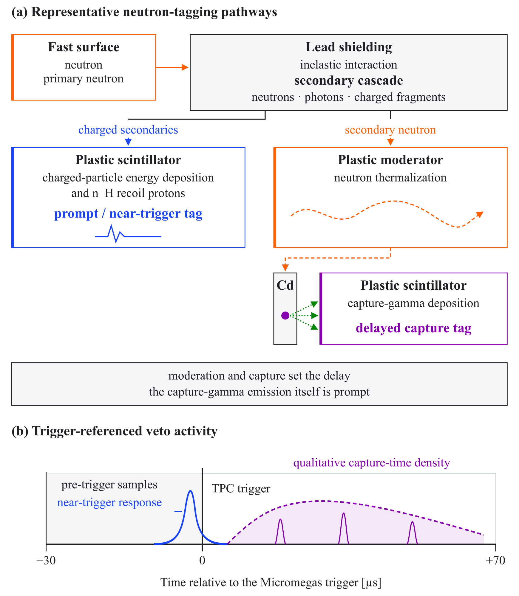
The central design principle is to tag the neutron-induced cascade rather than the incoming neutron. Fast primaries interact in the lead and copper, producing softer neutrons, photons, recoil nuclei, and charged fragments. Plastic scintillator samples the prompt charged component and moderates part of the neutron population. Cadmium sheets between active stages then capture a fraction of the thermalized component and emit gamma cascades close to a neighboring scintillator.
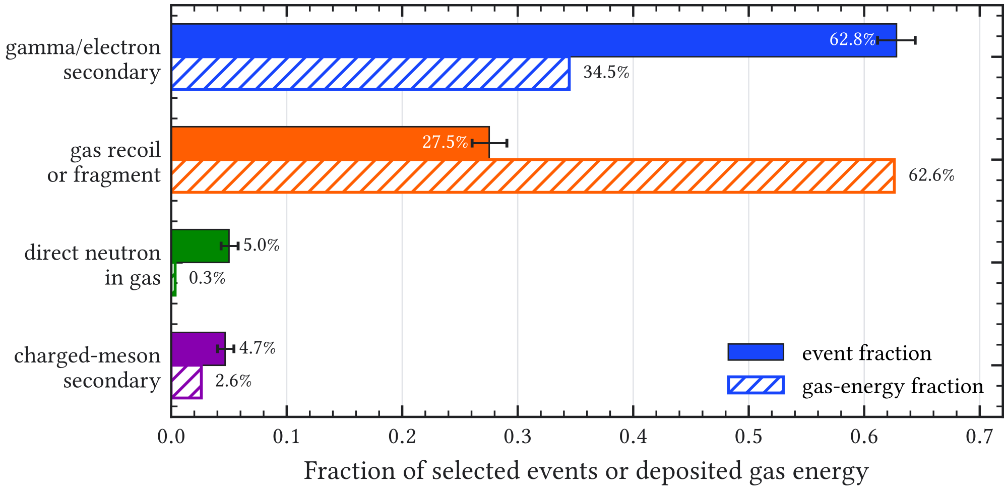
The need to tag this surrounding history is visible directly in the saved-event truth record. In a sample of 879 neutron-induced events with a TPC energy deposit, electromagnetic descendants account for 552 events (62.8%), gas recoils or nuclear fragments for 242 (27.5%), charged-meson descendants for 41 (4.7%), and direct neutron interactions in the gas for only 44 (5.0%). Thus, in almost two thirds of this sample the low-energy TPC activity is produced through the electromagnetic branch of a wider neutron-induced cascade. The classification is used only to establish the mechanism; it is neither an experimental particle label nor a source-normalization factor.
Simplified sandwich scans were used to establish where the active material should sit relative to the lead. The response was evaluated after Birks quenching in the scintillator, so the threshold represents an electron-equivalent visible-energy proxy rather than unquenched deposited energy [109, 110]. The full material-ordering and quenching diagnostics are preserved in Appendix Section A.7.
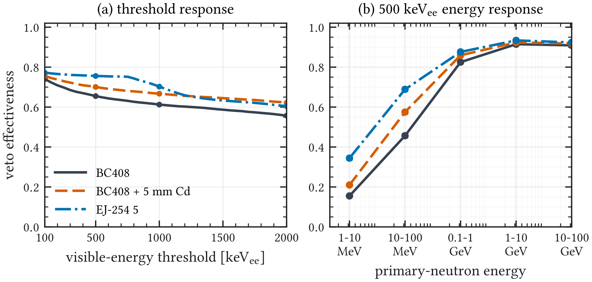
The bare scintillator responds most readily to neutrons that can interact directly in the active material. For the harder primaries that dominate Micromegas-triggering events, lead-coupled arrangements retain the useful response because they sample the secondary cascade. This is why the veto surrounds the passive shield instead of replacing it.
5.3.3 Transport-validation envelope
The two transport steps most directly connected to the design conclusion were checked independently. First, a thin-target benchmark of outgoing neutrons from natural lead at was compared with EXFOR data in the measured energy and angular acceptance. The four tested high-precision Geant4 reference lists lie – below the experimental integral and differ from one another by less than 1% in this low-energy benchmark. This agreement supports the secondary-shower interpretation, although it does not by itself validate the full GeV-scale HENSA response.
Second, alternative cadmium de-excitation treatments were replayed through the same detector-response and peak-finding chain. The probability of reconstructing any veto peak remains between 0.719 and 0.742, whereas the conditional fraction above the -equivalent operating point changes from 0.314 to 0.383. The existence of a neutron-sensitive signature is therefore more stable than its efficiency at a fixed reconstructed-energy threshold. The full cross-section comparisons, outgoing-neutron spectra, cadmium line yields, and response tables are retained in Appendix Section A.2; the threshold dependence enters the systematic envelope rather than being tuned to data.
5.3.4 Prompt and post-trigger signatures
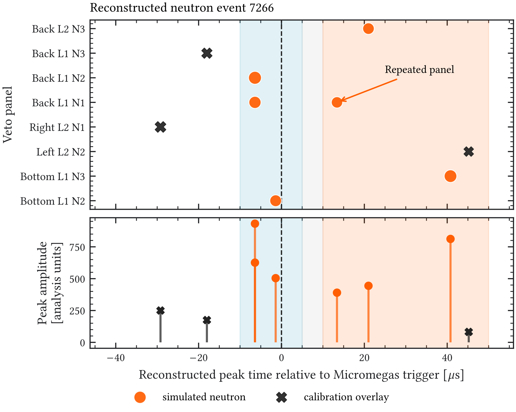
Here, prompt and post-trigger refer to time relative to the Micromegas trigger, not to the duration of the nuclear de-excitation. Figure 5.8 connects the simulated capture history to reconstructed veto activity.
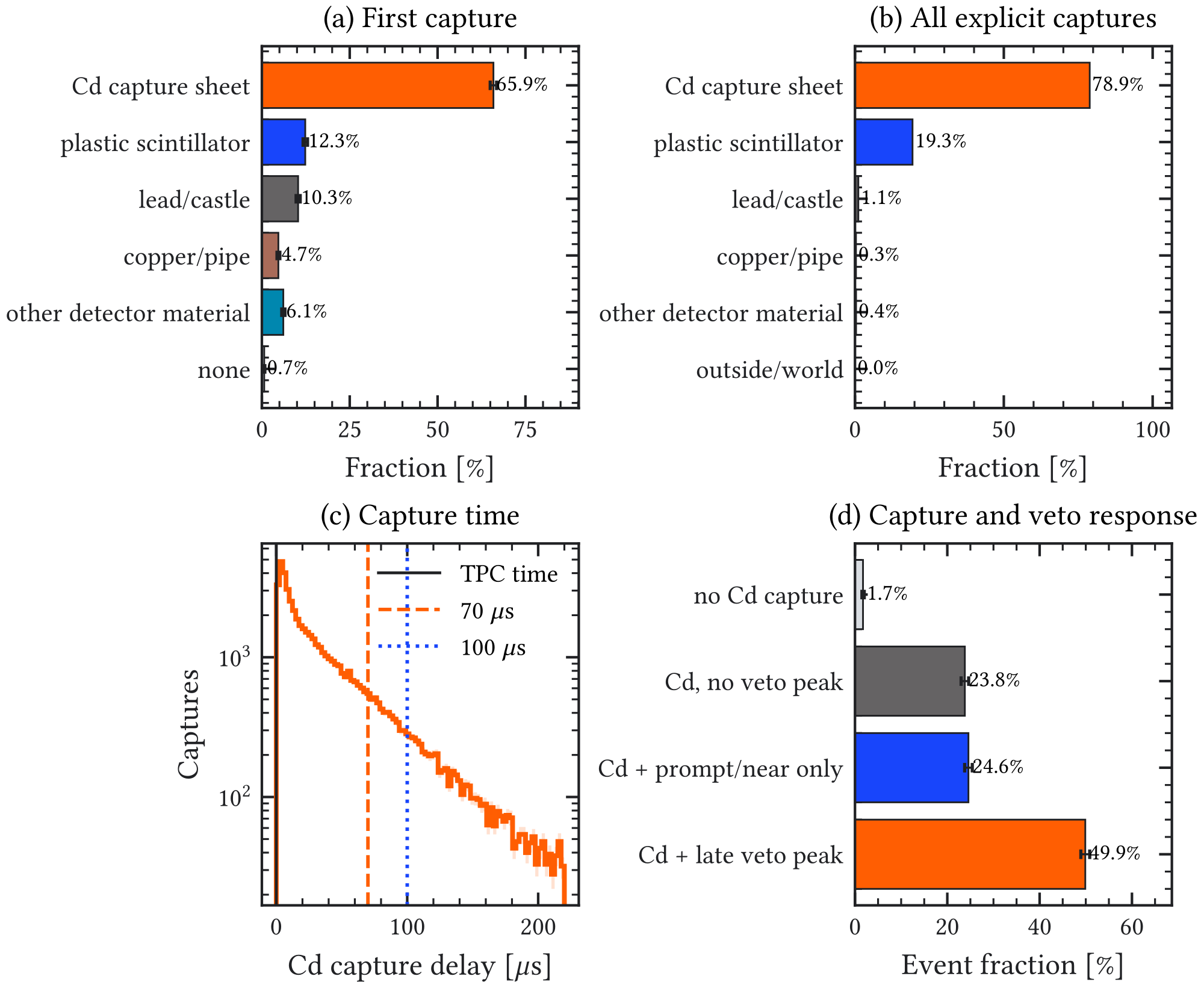
In the processed three-layer HENSA sample, 98.3% of analysis entries contain a cadmium-sheet capture and 78.9% of all explicit captures occur in cadmium. At event level, however, 23.8% contain a cadmium capture but no reconstructed veto peak. Approximately one quarter contain only prompt or near-trigger activity, while 49.9% contain a late reconstructed peak. Finite light collection, thresholds, timing, and reconstruction therefore prevent a one-to-one mapping between capture and observed veto signature.
The cadmium capture history in the HENSA three-layer simulation provides the characteristic post-trigger timescale relative to the first simulated gas deposit, which is used as a trigger proxy and is distinct from both the physical capture time and the reconstructed veto-peak time. A truncated-exponential fit to the selected post-trigger physical-capture tail gives . This is a simulation-derived capture-retention study, not a complete acquisition-window optimization: reconstructed thresholds, accidental activity, and dead time are not included in the fitted curve.
![Figure 5.9: Simulation-derived cadmium-capture timing and conditional retention for the HENSA three-layer sample, measured from the first simulated gas deposit used as a trigger proxy. Of the selected positive-delay captures, 79.7 % occur by 70 mus and 88.8 % by 100 mus . The published prototype record spans approximately [ − 30 , + 70 ] 𝜇 s relative to its hardware trigger; mapping that trigger to the gas-deposit proxy is a separate response requirement. These truth-history fractions are not reconstructed veto efficiencies. The denominator and fit interval are documented in Appendix Section A.4 .](assets/8f1a33ab1ea7ea056e7e892b.png)
Late-window activity alone is not neutron-specific because calibration data contain electronic noise and unrelated environmental coincidences throughout the waveform. The useful observable combines prompt or near-trigger activity with post-trigger energy, peak multiplicity, signal quality, and segmentation. An event-mixing study quantifies the timing information: a late peak alone accepts approximately 52% of the neutron sample and 56% of a neutron-derived time-scrambled control, whereas requiring both prompt and late activity accepts approximately 46% and 14%, respectively. The scrambled control preserves neutron-like peak multiplicity and amplitude while removing alignment to the trigger; it does not measure the apparatus’s accidental-coincidence rate. The improvement comes from the timing context rather than from late activity by itself; the capture-denominator bookkeeping, full trade-off plot, and selection definitions are documented in Appendix Section A.4. In this chapter, post-trigger or late-window activity always refers to peaks inside the recorded waveform. The term delayed activation is reserved for radioactive-decay descendants occurring beyond the coincidence window, as defined in Section 6.7. No standalone peak-multiplicity requirement is adopted as an operating point in this thesis. Multiplicity enters the structured and multivariate selectors together with energy, timing, channel occupancy, and signal quality; the final threshold is fixed by calibration-like control acceptance.
5.4 Multilayer optimization
The design scan compares one-, two-, three-, and four-layer cadmium configurations, together with three-layer gadolinium and stainless-steel variants. The HENSA outdoor neutron field is propagated through the full detector-response chain, including quenching, light attenuation, waveform formation, and veto-peak reconstruction. The scan exporter retains every entry in each processed AnalysisTree; it applies no additional one-track, –, fiducial, or X-ray-topology selection. The denominator is therefore a response-level analysis-entry population, not the conservative reference selection of Section 6. All efficiencies in this section are conditional on that exported population.
The distinction between performance quantities is essential. The probability of any reconstructed veto tag tests whether the geometry produces an observable response. Threshold rejection tests a particular visible-energy operating point. The aggregate classifier adds multiplicity and signal-quality information at a fixed calibration acceptance. None of these conditional quantities is an absolute neutron background level.
| Quantity | Denominator | Noise / acceptance treatment | Purpose |
|---|---|---|---|
| Any veto tag | Exported HENSA AnalysisTree entries | No accidental overlay | Geometry response |
| threshold rejection | Same response-level sample | Reconstructed visible-energy proxy; no accidental overlay | Comparable layer operating point |
| Aggregate classifier rejection | Three-layer response sample with calibration-noise overlay | Threshold fixed at calibration-like control acceptance | Overlaid design diagnostic |
| Absolute background level | Generated exposure and source normalization | Source-appropriate veto credit with prompt/delayed split | Reported in Section 6 |
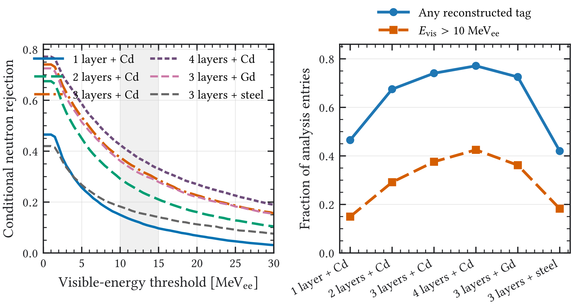
The any-tag fraction increases from for one layer to , , and for two, three, and four cadmium layers, respectively. At a -equivalent threshold, the corresponding conditional rejections are , , , and . Thus the third layer provides a substantial improvement, whereas the fourth adds in any-tag probability and in threshold rejection while increasing the channel count from 59 to 79. The gadolinium variant is similar to cadmium for these aggregate observables, whereas stainless steel provides substantially weaker tagging.
Generated-primary normalization gives a processed-analysis-entry probability of approximately for each of the one- through four-layer cadmium samples. The active layers improve the conditional tagging response; within the statistical precision of this diagnostic, they do not reduce the population reaching the response-level analysis denominator. The exposure audit and full diagnostic projections are given in Appendix Section A.8.
Each additional layer also adds channels that can contribute accidental activity. An illustrative overlay model samples the measured calibration-triggered veto activity and scales the number of independent accidental opportunities with the active layer count. It is used to expose the trade-off, not as a final dead-time measurement.
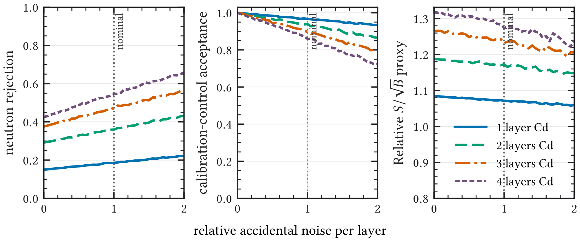
The accidental-overlay model does not, by itself, favor three layers: over the scanned noise range, the four-layer configuration retains the largest simple sensitivity proxy. At the nominal scale, that proxy is for four layers and for three layers, while the corresponding calibration-like control acceptances are and . Three layers are therefore an engineering and channel-count compromise made after most of the conditional tagging gain has been obtained, not a statistical optimum of this simplified model. The small separation between the three- and four-layer sensitivity proxies should be compared with the response and cascade-model variations before assigning a preferred physics operating point. For an expected background of only a few counts, an expected Poisson-likelihood limit with signal and live-time losses is more appropriate than .
5.5 Prototype geometry and synchronized readout
5.5.1 Geometry and prototype construction
The 59-panel simulated design is organized into Top, Bottom, Left, Right, Front, and Back groups, with three active stages per group. The nominal symmetric arrangement would contain 60 panels, but one short inner-top panel is absent to accommodate mechanical and service constraints. Thin cadmium sheets are placed between neighboring active stages so that moderated neutrons can capture near a scintillator.
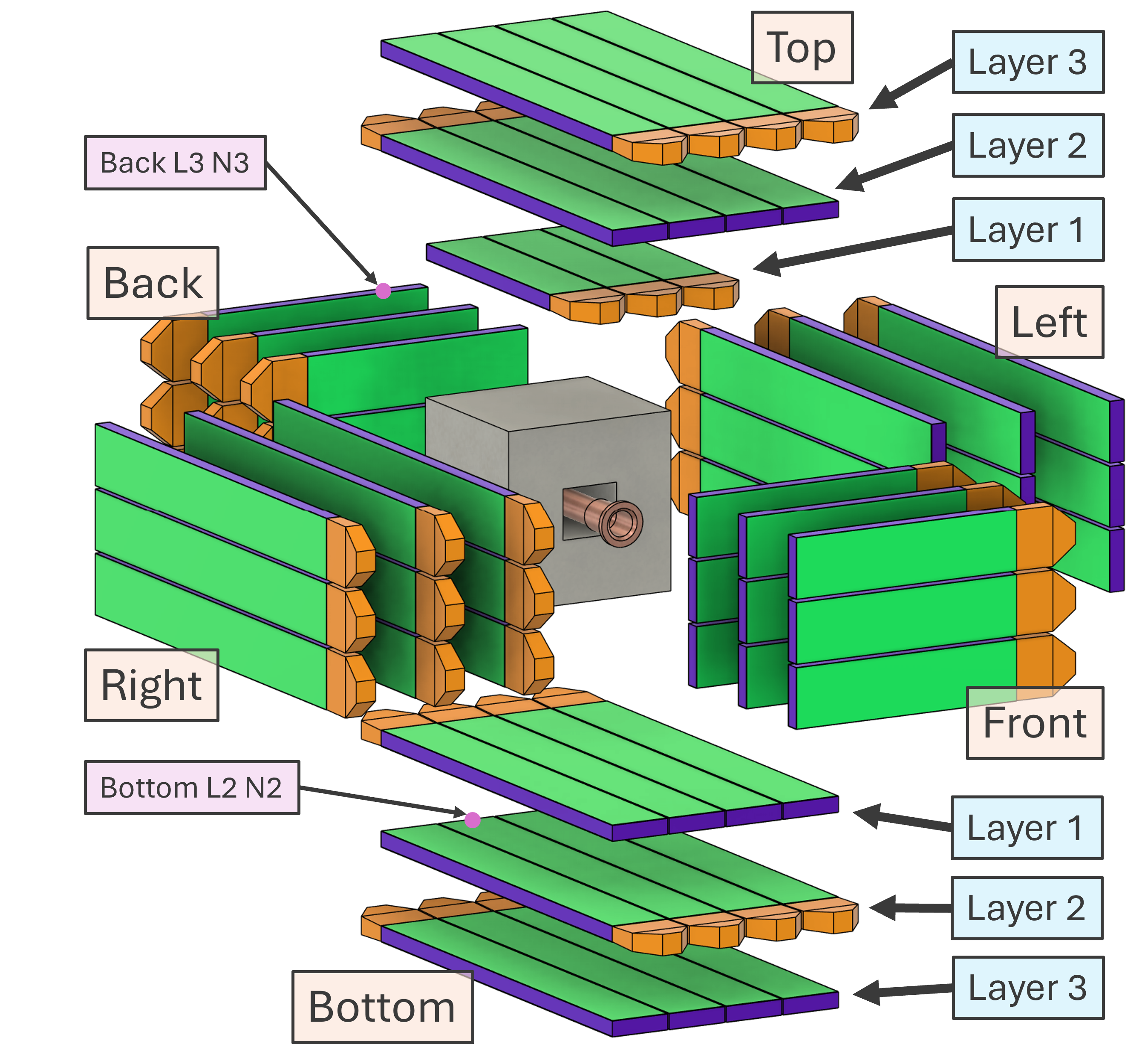
| Group | Layers | Panels per layer | Lengths | Design note |
|---|---|---|---|---|
| Top | 3 | 3 / 4 / 4 | 80 / 150 cm | One short inner panel is omitted, giving 59 rather than 60 panels. |
| Bottom | 3 | 4 / 4 / 4 | 150 cm | Full long-panel coverage below the detector. |
| Left | 3 | 3 / 3 / 3 | 150 cm | Long side coverage. |
| Right | 3 | 3 / 3 / 3 | 150 cm | Long side coverage. |
| Front | 3 | 3 / 3 / 3 | 80 cm | Short modules on the beam-pipe side. |
| Back | 3 | 3 / 3 / 3 | 80 cm | Short modules on the rear side. |
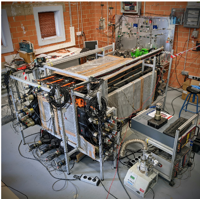
The prototype reused NE-110 plastic scintillator bars from a former time-of-flight spectrometer [111]. The bars were cut to and , with a cross-section, and coupled to photomultiplier tubes through light guides. The physical prototype used cadmium sheets between neighboring panels and layers, realizing the same capture-stage concept as the simulation [17]. Atmospheric muons provided the gain-equalization reference. For a flat plastic panel, the most probable through-going-muon signal corresponds to approximately of visible energy; this anchors the –-equivalent region used in the threshold studies [17]. Measurements on the long bars showed that the collected light at the far end can be reduced by approximately a factor of two, so the reconstructed energy is an attenuation- and calibration-dependent proxy rather than a local calorimetric measurement [17].
5.5.2 Electronics and timing
The Micromegas and veto branches each use four AGET application-specific integrated circuits and are synchronized by a common trigger and clock [17, 81]. The circular buffer contains 512 samples, allowing the trigger position and window length to differ between detector branches. For the prototype-like veto configuration, the total acquisition is with the Micromegas trigger after the start. The trigger-centered convention used below is therefore approximately : near-zero activity provides the prompt tag, while capture-related peaks at positive times contribute to the post-trigger tag only if they occur before the waveform boundary.
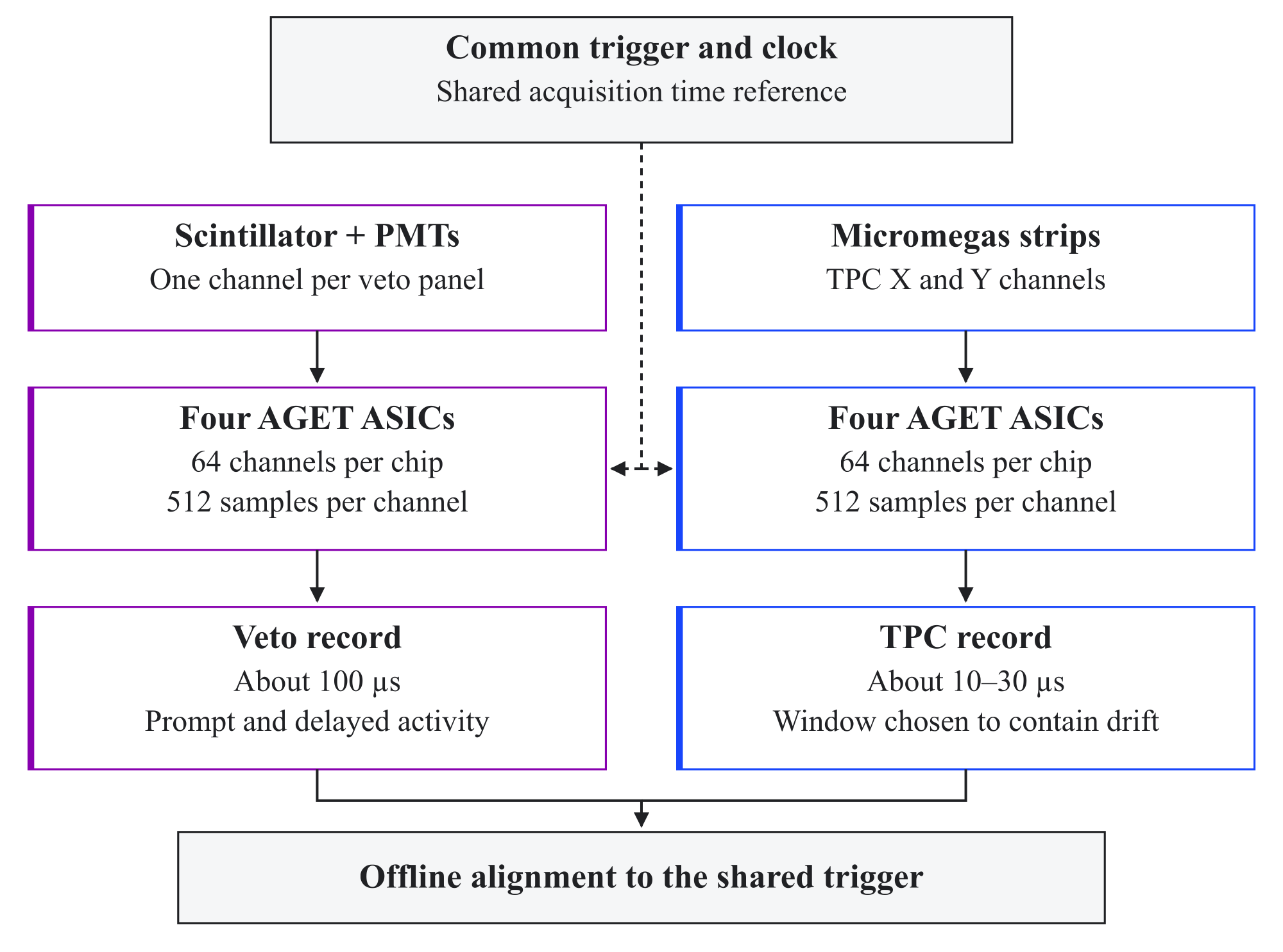
The long veto window is a deliberate part of the neutron-sensitive design. It retains prompt muon and shower activity as well as a substantial fraction of the cadmium-capture tail. The window cannot be widened on capture retention alone, because every additional interval also increases random-coincidence and live-time costs.
5.6 Waveform observables and conditional performance
5.6.1 Detector response and reconstructed observables
The simulation is propagated beyond deposited energy to the quantities used in data. Energy deposits are quenched, attenuated according to their propagation distance, converted into channel signals, shaped, digitized, and processed by the REST peak finder. This common representation permits the same peak time, amplitude, multiplicity, and channel-quality definitions to be used for simulated and experimental events. The common reconstruction-process inventory is given in Table A.1, while veto-specific campaign and response settings are documented in Appendix Section A.6.
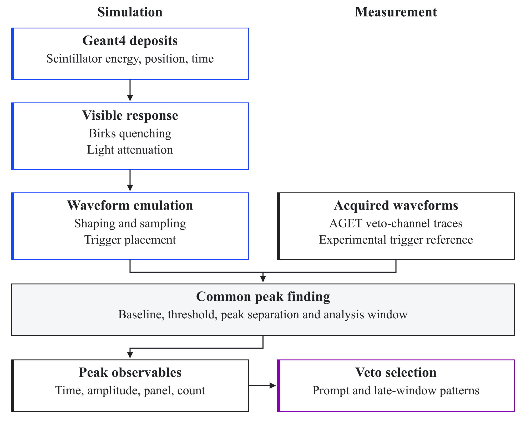
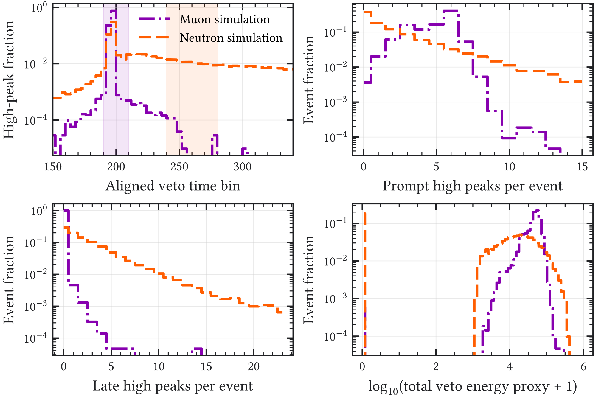
Geant4 deposits to analysis-level veto observables. Quenching, light attenuation, waveform formation, and peak reconstruction are included before the veto decision.Muon-induced events are predominantly prompt, high-amplitude, and track-like across several panels. HENSA neutron-induced events are more heterogeneous: they contain softer prompt activity, a broader post-trigger tail, and less regular channel correlations. These differences motivate aggregate observables rather than a single opposite-panel coincidence.
5.6.2 Calibration-controlled classifier hierarchy
An initial design-facing classifier combined five aggregate reconstructed quantities and established that waveform multiplicity and signal-quality information outperform a single visible-energy threshold. That event-random study is retained in Appendix Section A.4 as a historical benchmark. The run-disjoint study uses the higher-statistics aligned sample of 20,274 HENSA neutron events and 139,454 experimental calibration events. One independently sampled calibration peak train is concatenated with each simulated neutron peak train. This preserves correlations within the measured activity but does not reproduce peak merging, saturation or baseline shifts that can occur when waveforms overlap before peak finding. The control class is the calibration-triggered activity itself, and every score is treated as an ordering variable rather than an event-by-event neutron probability.
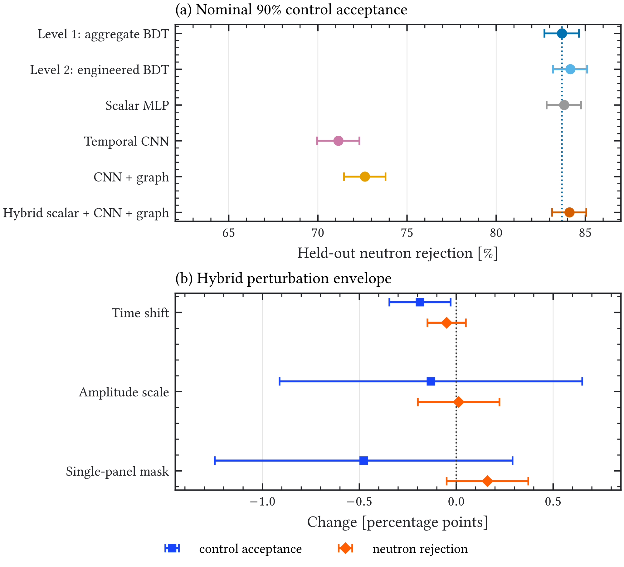
The analysis is organized into three implemented levels of increasing opacity. The level-1 boosted decision tree uses six directly interpretable aggregate observables: total reconstructed veto-energy proxy, peak count, unique panel count, active face count, active layer count, and maximum peak amplitude. The level-2 model adds disjoint waveform-window summaries, face and layer occupancies, amplitude fractions and entropies, opposite-face activity, and face–time and layer–time interactions. The level-3 model replaces these engineered spatiotemporal quantities with a two-channel panel–time representation and combines a shared temporal convolution, a relational panel graph, attentive pooling, and the six level-1 aggregates. No Micromegas energy or topology observable enters any level of this classifier hierarchy. Simulation and prototype channel identifiers are first mapped with separate readout maps to a common coordinate; this prevents identical electronic identifiers in the two readouts from being assigned to different physical panels after noise overlay.
The partition is chronological and run-disjoint. Calibration runs 1335, 1339, and 1342 train the models, run 1345 fixes the score thresholds at nominal 90% and 95% control acceptance, and run 1347 is used once for the held-out evaluation. An overlaid neutron event follows the partition of its sampled calibration event, preventing empirical-noise leakage. The mapped waveform coordinate is divided into pre-control bins 0–189, prompt bins 190–210, early post-trigger bins 211–239, capture bins 240–280, and late-tail bins 281–511. The following hierarchy results retain the original response and feature definition as a historical comparison. A subsequent boundary check rejects peaks outside the stored 512-bin record instead of clipping them to its endpoints; the bounded frozen-model comparison is given in Appendix Section A.4.1.1. The physical acquisition support and calibrated total-energy response remain unresolved for this flat input, so the comparison does not establish an absolute neutron-veto efficiency.
| Classifier | Inputs | Held-out AUC | Neutron rejection at nominal 90% control acceptance |
|---|---|---|---|
| Level 1: aggregate | 6 | 0.911 | |
| Level 2: aggregate + time | 43 | 0.913 | |
| Level 2: aggregate + capture delay | 24 | 0.913 | |
| Level 2: aggregate + position | 49 | 0.912 | |
| Level 2: full spatiotemporal | 164 | 0.911 | |
| Level 3: hybrid neural model | tensor + 6 | 0.913 | |
| Full model without total energy | 163 | 0.896 |
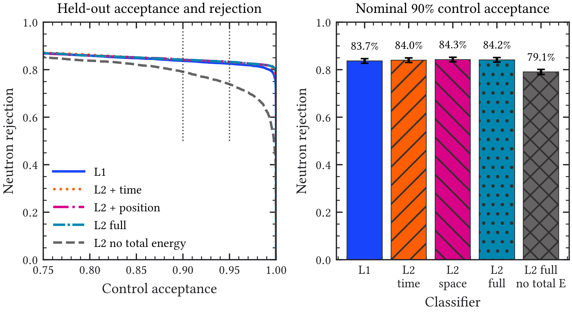
The full level-2 model improves the held-out rejection by only 0.47 percentage points relative to level 1, with a central 90% paired-bootstrap interval of 0.07–0.82 percentage points, while its AUC difference is consistent with zero. Moreover, the nominal level-1 calibration acceptance varies from 88.2% to 90.9% across the five runs, whereas the full model varies from 84.4% to 90.5%. The added dimensions therefore amplify one run-dependent control shift without producing a material rejection gain. The total-energy removal test retains 79.1% rejection, demonstrating that timing and position contain independent neutron-sensitive information, but permutation tests show that total visible energy remains the dominant nominal input. Level 1 is consequently retained as the reference classifier for this historical response study; the additional levels test information content without establishing a more robust physical operating point.
5.6.2.1 Capture-delay signature
The small gain from the generic timing vector does not imply that neutron-capture timing is physically uninformative. It answers a narrower question: once total reconstructed veto energy, amplitude, and multiplicity are known, the original broad waveform summaries add little to the global binary classifier. The delayed-capture hypothesis is therefore tested separately, distinguishing the physical capture time from the reconstructed peak time and from an accidental late pulse.
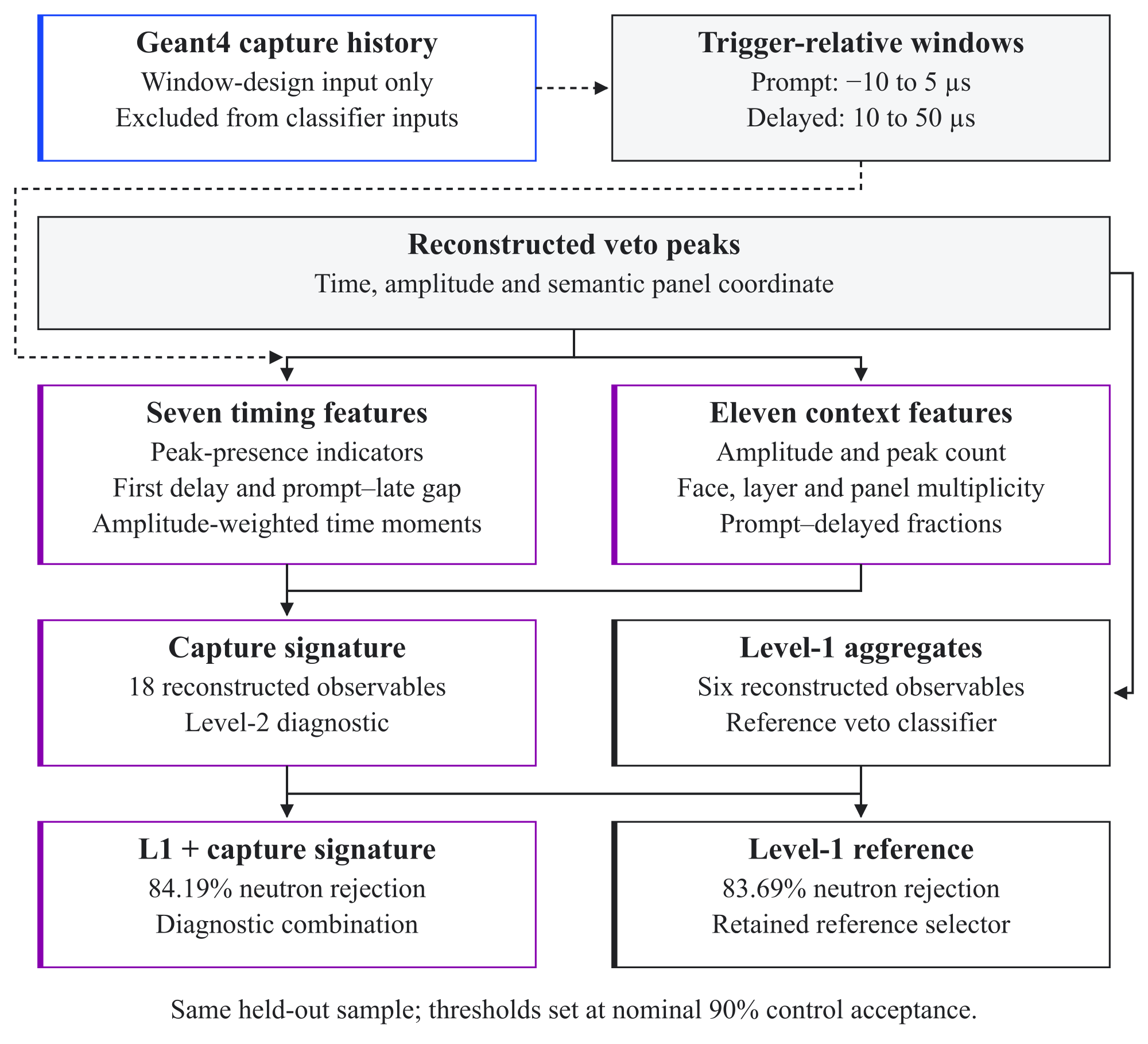
Geant4 truth is used only to establish the expected timescale. For 55,581 positive-delay cadmium captures in the three-layer HENSA sample, the median delay from the first gas deposit is , and a truncated-exponential fit to the – tail gives . The cumulative fractions captured after the trigger and no later than , , and are , , and , respectively, using all records with as the denominator. The narrower observable interval contains of those records; another occur within the first and are not part of the delayed window. This truth information fixes the physical interpretation and the candidate window; it is never supplied to an event classifier.
The historical feature construction maps waveform bin to an aligned time coordinate through
(5.1)
The offset 231 aligns prompt populations empirically; it is not an independent calibration of the hardware-trigger position. In this coordinate, bins 0–511 span , whereas the simulated peak population in the inspected flat neutron input ends at . Consequently, the nominal capture-like interval below is only partly populated by physical simulated peaks; calibration overlay can still populate its remaining bins. The observable prompt interval is , while the capture-like interval is . The gap separates the nominal prompt and delayed intervals, but does not by itself bound pulse tails or peak-finding leakage. The explicit timing coordinates are the first delayed-peak time, the interval from the last prompt peak to the first delayed peak, and the delayed amplitude-weighted time mean and width. Binary indicators record whether prompt and delayed peaks exist, so the numerical zero assigned to a missing time coordinate cannot be interpreted as a physical zero delay. The capture-like signature then adds prompt and delayed multiplicities and amplitudes, panel, face, and layer occupancies, delayed fractions, and the number of panels that become active only after the prompt interval.
A time-scrambled event-mixing test isolates the importance of the sequence. It draws complete veto-peak trains from other simulated neutron events and circularly shifts them within the acquisition interval, preserving energy, multiplicity, and spatial correlations while destroying their timing relation to the Micromegas trigger. This neutron-derived null tests the timing sequence; it does not bound the experimental accidental rate. The resulting trade-off is summarized in Table 5.5.
| Observable requirement | Neutron acceptance | Time-scrambled acceptance | Ratio |
|---|---|---|---|
| At least one – peak | |||
| Prompt followed by a – peak | |||
| Prompt + delayed activity in at least two veto groups | |||
| Previous row + delayed peak-energy proxy above analysis units |
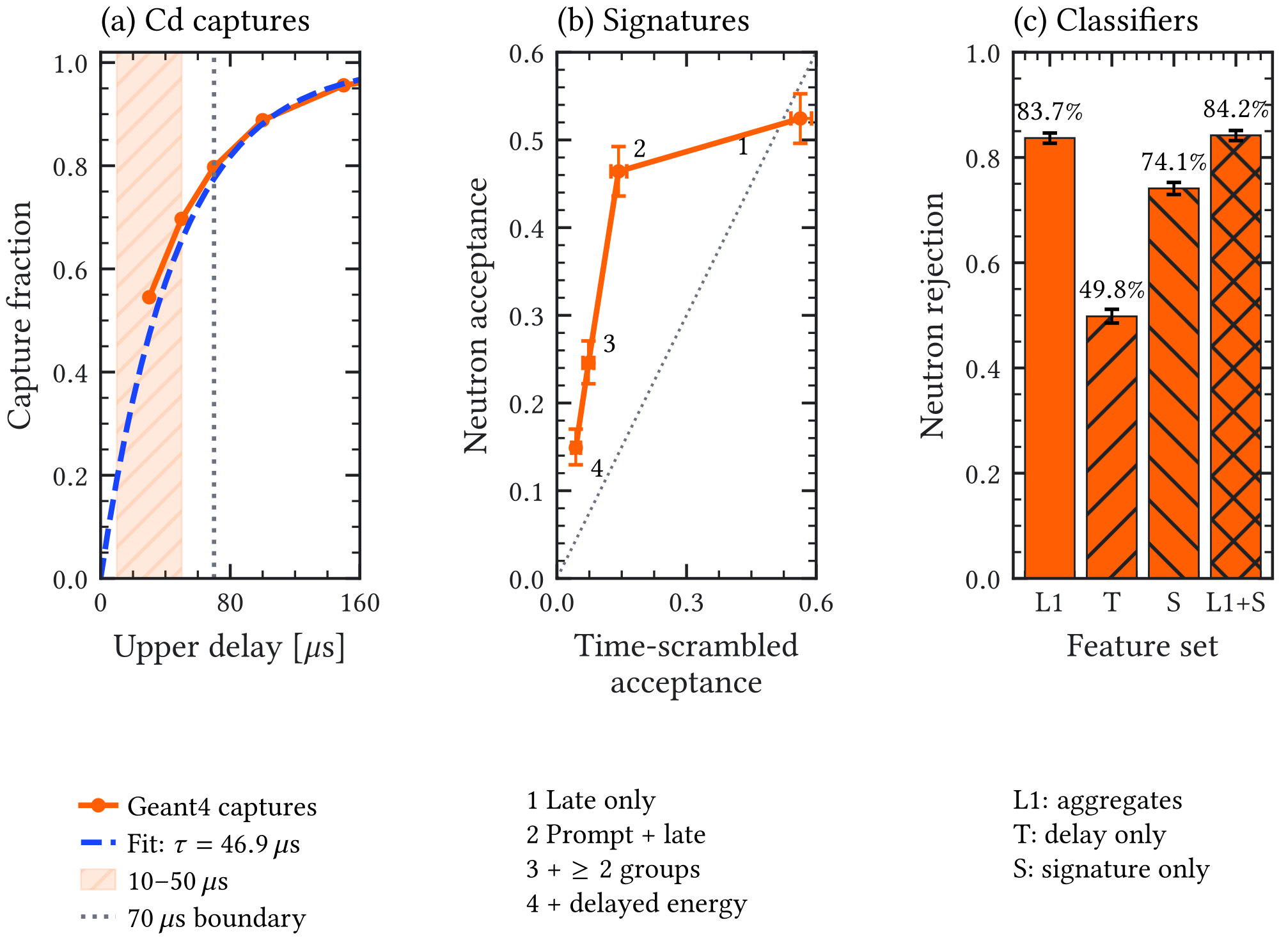
The seven delay coordinates alone reject of the held-out neutrons, and the complete 18-variable capture signature rejects . Thus, capture timing is informative but is not a universal neutron tag: of the selected events containing a truth-level cadmium capture have no reconstructed veto peak ( of all selected events), and late activity also occurs in calibration data. Adding the capture signature to the six level-1 aggregates raises the held-out rejection from to , corresponding to 20 additional rejected neutrons among 4035. The paired-bootstrap gain is percentage points, with a central 90% interval of – percentage points, whereas the AUC difference remains compatible with zero. The minimum control acceptance across the five runs decreases from for level 1 to for the combined model. The delay is therefore retained as an important, physically interpretable level-2 signature and as a central input to the sequence model, while the aggregate level-1 BDT remains the nominal selector.
5.6.2.2 Level-3 spatiotemporal neural model
The level-3 input has shape : for every common semantic panel and aligned waveform bin, the two channels contain summed peak amplitude and peak occupancy. The simulation-only panel absent from the prototype is masked, and no run identifier, raw channel identifier, overlay identifier, TPC quantity, or Geant4 truth enters the network. A shared temporal convolution encodes each panel; two graph blocks exchange information separately between same-face neighbors, adjacent layers, and opposite faces before attentive pooling. Four predeclared variants distinguish a scalar multilayer perceptron, a tensor-only temporal convolution, a tensor-plus-graph model, and the final hybrid with the six level-1 aggregates.
The tensor-only models reject only 71.2% and 72.6% of the held-out neutrons, respectively, showing that the present sparse peak tensor does not replace the global energy summaries. The hybrid reaches 84.1%, only 0.42 percentage points above level 1; the central paired-bootstrap 90% interval is 0.10–0.74 percentage points, while the AUC difference remains compatible with zero. The frozen score is insensitive at the sub-percentage-point level to shifts of up to five waveform bins and to 10% amplitude rescaling in neutron rejection. Masking one representative panel per face–layer cell changes the rejection by at most 0.37 percentage points, but can reduce control acceptance by 1.25 percentage points. Most importantly, the nominal 90% control acceptance falls to 83.4% in calibration run 1339, below the 84.4% minimum of level 2 and the 88.2% minimum of level 1. The neural model therefore confirms the performance ceiling without satisfying the predeclared run-stability gate.
The frozen level-1 model is then applied to the exact 249 conservative-reference HENSA candidates from Section 6.6.3. The three causal-history activation events are removed before prompt scoring and receive no veto credit. For each of the remaining 246 candidates, 200 independent calibration events are overlaid. The mean prompt rejection is 91.14%, leaving 21.8 candidates on average; the central 90% range over accidental overlays is 19–25 survivors. The reproducible first overlay realization leaves 22 candidates, corresponding to with a two-sided 90% Garwood interval. The full level-2 model leaves 20.6 candidates on average, a reduction of only 1.2 events relative to level 1. The level-3 hybrid leaves 21.0 candidates on average, with a central 90% overlay range of 18–24, and the first realization leaves 20. This is less selective than level 2 and only 0.8 event below level 1, so it does not alter the controlling prompt-background estimate. The delayed-activation channel remains separate at the one-sided saturation bound reported in Section 6.7. The training, readout maps, run partitions, fixed models, candidate identities, and overlay draws are documented in Appendix Section A.4.
5.7 Experimental validation with IAXO-D0
5.7.1 Published surface cut flow
The commissioned prototype was operated with IAXO-D0 at surface level in Zaragoza for an effective [17]. The published selection uses a – region of interest and a -radius focal region. This should not be confused with the fiducial radius used by the current conservative background-analysis contract.
| Stage | Selection | Events | Background level |
|---|---|---|---|
| Raw acquisition | Full detector and energy range | 1,305,996 | – |
| Micromegas selection | –, focal region, X-ray-like topology | 257 | – |
| Prompt veto | Prompt muon-like veto discrimination | 56 | |
| Advanced veto | Multiplicity and activity in prompt and post-trigger sub-windows | 49 |
The prompt selection removes of the Micromegas-selected events and is the dominant surface-background rejection. The advanced selection removes of the post-prompt sample; the exact two-sided 90% binomial interval is –. The calibration efficiency after all cuts is relative to the Micromegas-selection reference. No separate prompt-stage calibration efficiency was reported, so this ratio is not described as retention relative to the prompt veto.
Figure 5.21 replots the reported cut-flow values in a terminology consistent with the present analysis. The stage historically called a “neutron cut” is labeled a neutron-sensitive control selection because the data do not establish the origin of individual rejected events.
![Figure 5.21: IAXO-D0 surface cut-flow summary reconstructed from the published event counts and background levels in Ref. [ 17 ]. Panel (a) shows the cumulative candidate population after the Micromegas, prompt-veto, and advanced veto selections. Panel (b) gives the corresponding exposure-normalized background levels after the two veto stages, with exact 90% Poisson intervals. The final stage is described as a neutron-sensitive control selection; it does not provide event-by-event neutron identification.](assets/f110b21886ee47e240f63059.png)
The data support the hierarchy expected from the design. Prompt activity provides the large muon-like rejection, and the long waveform supplies an additional handle on non-prompt or multiplicity-rich activity with a small calibration penalty. The seven additionally rejected events do not measure a neutron efficiency because the post-prompt sample contains an unknown mixture of neutron-induced, proton-induced, environmental, activation, and instrumental backgrounds.
5.7.2 Late-window control population
An exploratory thesis extension ranks the feature-complete flattened prototype sample against calibration accidentals, muon simulation, and HENSA-neutron simulation. After removing prompt-muon-like and burst-like events, a frozen score orders the remaining events by their similarity to the neutron-plus-noise template relative to calibration and muon controls. Its threshold is fixed at the upper 1% tail of the clean calibration distribution. The score is deliberately used as a control-population selector rather than as an event-by-event neutron probability; its exact construction, preprocessing, and time-window definitions are documented in Appendix Section A.5.
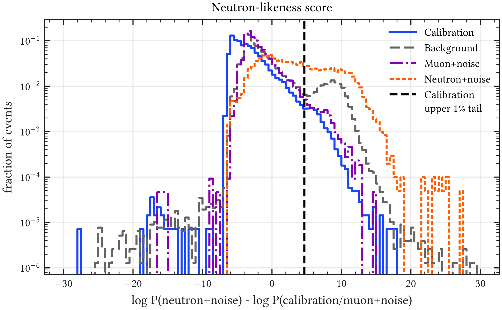
| Sample | Events | Prompt tag | Clean after prompt | Median score | Selected |
|---|---|---|---|---|---|
| Calibration | 139454 | 11.00% | 123441 | 1235 | |
| Flat experimental background | 777752 | 91.13% | 65990 | 3877 | |
| Muon+noise simulation | 21569 | 97.98% | 433 | 12 | |
| Neutron+noise simulation | 20274 | 51.95% | 9697 | 1722 |
The score selects 3877 experimental events, corresponding to 0.50% of the full flattened input and 5.88% of its prompt-suppressed subset. The selected data differ from the calibration control and have passed prompt-muon-like rejection, but they are not quantitatively described by the present HENSA template. In particular, their veto multiplicity, late-window energy, and Micromegas topology differ substantially from the selected neutron-plus-noise simulation. The defensible result is therefore the observation of a calibration-controlled late-window population, not a neutron fraction or a background-model normalization. The detailed template-mismatch table and channel correlations remain in Appendix Section A.5; the event rasters and Micromegas projections are collected in Appendix Section A.10.
5.7.3 Limits of experimental neutron identification
The frozen score identifies an experimentally distinct population enriched in neutron-sensitive observables, but it does not identify a sample of neutrons with known purity. At the threshold accepting of the clean calibration control, of the prompt-suppressed background population is selected. This establishes a difference between the score distributions of background and calibration events. The score also contains Micromegas energy, and its overlapping time windows and run-dependent control populations can produce a difference without a unique new particle component. The comparison therefore does not exclude ordinary accidental or instrumental explanations and does not establish individual event origins.
The principal obstacle is the quantitative mismatch with the available neutron template. The selected data contain a median of 47 reconstructed veto peaks, compared with 9 in the selected neutron-plus-noise simulation, and their median late-window energy proxy is approximately 2.5 times larger. Their Micromegas energy, hit multiplicity, and topology also differ substantially. Consequently, interpreting all selected events as neutrons would contradict the measured observables, while converting the selected count into a neutron rate would import an unsupported template-purity assumption.
Several effects prevent a stronger attribution in the present study. No neutron-source or otherwise tagged neutron data are available for the commissioned configuration. The HENSA production represents an outdoor spectral model rather than a run-matched experimental calibration, and the 59-panel simulation does not reproduce every gap, threshold, gain, unstable channel, and time-dependent condition of the 57-panel prototype. The experimental sample can also contain residual proton- and photon-induced showers, activation products, correlated electronics activity, and other instrumental populations for which complete normalized templates are not available. Finally, a late peak is not neutron-specific: accidental activity is common, and long-lived activation is causally distinct from an in-waveform capture response.
The existing data can strengthen the control result through run- and channel-state matching, matching in Micromegas energy, a veto-only score, and time-shifted or off-time control windows. Score construction and threshold setting should use different runs from the comparison sample. A quantitative neutron fraction would additionally require credible competing templates and independent particle-response constraints, for which tagged neutron data would be particularly useful. Until these conditions are met, the thesis reports a calibration-controlled, neutron-sensitive late-window population rather than an observed neutron count.
5.8 Systematic limitations
| Uncertainty class | Consequence for the veto conclusion |
|---|---|
| Surface neutron field | HENSA constrains the Zaragoza outdoor field; transfer to the planned DESY installation remains site dependent while the detector and site contracts are not frozen. |
| Hadronic and capture models | Lead secondary production and cadmium gamma partition alter threshold-dependent response. The tested replay gives a model spread; its coverage of thermal transport, the frozen classifier and GeV-scale layer ordering is incomplete. |
| Visible-energy response | Recoil identity and true step length are not fully represented by the historical quenching approximation. Quenching, effective attenuation, gain and peak finding must be propagated to panel thresholds and selected candidates. |
| Geometry and channel state | The 59-panel simulation and 57-panel prototype differ in coverage, channel mapping, gaps, thresholds, and unstable-channel history. |
| Acquisition and accidentals | Peak-list overlays preserve measured control patterns but omit waveform overlap. Trigger mapping, physical record support, channel rates and online logic determine acceptance loss. |
| Experimental particle attribution | The late-window selection is enriched relative to calibration controls, but no tagged neutron sample or complete set of normalized competing templates is available. It therefore cannot determine neutron purity or rate. |
| Delayed activation | Long-lived radioactive descendants are not coincident with the initiating shower and cannot receive prompt-veto rejection credit. |
The background model also evaluates cosmic-induced random veto activity in a fixed simulated window, as described in Section 6.6.5. That result is distinct from a measured full-system dead-time estimate, which remains configuration dependent. The present chapter therefore reports calibration acceptance for offline selections and does not infer an unmeasured online live-time correction.
Detector inclination during solar tracking was tested separately for muons and HENSA neutrons. Across the simulated to range, the processed TPC-response acceptance varies at the few-percent level without a resolved monotonic trend. The scan in Appendix Section A.3 is conditional on its historical angular input; it does not close the final tracking-exposure dependence before that input is reconciled.
5.9 Summary and outlook
The shielding studies establish a coherent surface-detector strategy. Lead is indispensable for photon attenuation but does not remove the fast-neutron component; instead, it helps create the correlated secondary shower that an active system can tag. Passive borated-HDPE moderation improves selected configurations only modestly and cannot replace the veto.
The historical prototype design uses three scintillator–cadmium stages around the lead shield. The conditional HENSA response increases strongly through the second and third stages and only modestly in the fourth, while additional channels increase mechanical and accidental-veto costs. Generated-primary normalization shows no resolved reduction of the processed analysis-entry population across the one- through four-layer scan; the observed gain is additional reconstructed tagging information.
The IAXO-D0 data validate the two-level analysis logic. Prompt veto activity removes the dominant muon-like population, and late-window or multiplicity-rich waveform observables provide a smaller additional rejection while retaining of the Micromegas-selected calibration efficiency. The simulations establish neutron-sensitive response, whereas the prototype data demonstrate an additional non-prompt rejection handle without identifying the seven rejected events as neutrons. The extended data study similarly isolates a calibration-controlled population enriched in delayed and multiplicity-rich activity, but its mismatch with the HENSA template prevents an experimental neutron count or fraction from being inferred. The present experimental result is additional rejection with unresolved particle attribution. Absolute prompt and delayed background levels are evaluated by the source-normalized analysis in Section 6.
Within the historical simulation-based hierarchy, the six-observable aggregate boosted tree provides the reference result. The engineered timing and segmentation model confirms that these observables contain independent neutron-sensitive information, but its nominal rejection gain is only about half a percentage point and it is less stable across one calibration run. The completed neural study reaches the same conclusion independently: explicit temporal convolution and spatial message passing recover the aggregate performance only when the aggregate branch is restored, while the resulting gain is below one candidate and the run dependence worsens. Greater model complexity is therefore retained as a validation study rather than adopted as the nominal selector. The next useful simulations should first close recoil visibility, acquisition timing and source angular support, then propagate cascade and response alternatives through a frozen selector. A March 2026 collaboration design study explores compact three-layer modules with wavelength-shifting fibers and SiPM readout, including boron-loaded material and cadmium options [112]. That geometry should be compared with the historical PMT implementation under a common mechanical envelope and response model; single-bar test efficiency is not a measurement of complete-veto efficiency.