MEMORIA DE TESIS DOCTORAL
PROGRAMA DE DOCTORADO EN FÍSICA
2021–2024
_______________________________________________________________________
Simulation Infrastructure and Cosmic-Ray Background Modeling for
BabyIAXO Micromegas Detectors
REST-for-Physics/restG4 workflows, cosmic-neutron studies, and active-veto validation
______
Autor Luis Antonio Obis Aparicio
Directores Dra. Gloria Luzón Marco
Zaragoza, 2026
Abstract
BabyIAXO is the intermediate stage of the International Axion Observatory, a program to search
for solar axions through their conversion into X-rays in a strong magnetic field. Its planned surface
operation requires detectors that reject cosmic-ray backgrounds while retaining a weak keV X-ray
signal. This thesis develops simulation, background-modeling, and active-veto methods for the
IAXO Micromegas detector program.
The software work extends REST-for-Physics and its Geant4 interface, restG4,
through source generation, geometry construction, detector-response processing, and
large-scale simulation workflows. For IAXO-D1 operated with argon–isobutane, a source
inventory organizes cosmic, environmental, and intrinsic backgrounds under a common
reconstructed-event selection. Generated-primary counts and unresolved normalization
requirements are recorded explicitly. Tests of learned topology discrimination reveal substantial
simulation-to-data disagreement, so no learned rejection is credited in the reference
selection.
The shielding studies identify secondary showers produced by high-energy neutrons in lead as
an important background mechanism. They motivate a multilayer plastic-scintillator–cadmium
veto combining prompt activity with delayed capture signatures. Three layers provide a practical
compromise between conditional tagging performance and detector complexity. A quantitative
neutron efficiency still requires validation of waveform acceptance, quenching, and capture
modeling. Neutron-induced activation is evaluated separately through production and
radioactive-decay simulations, without assigning prompt-veto suppression to delayed
decays.
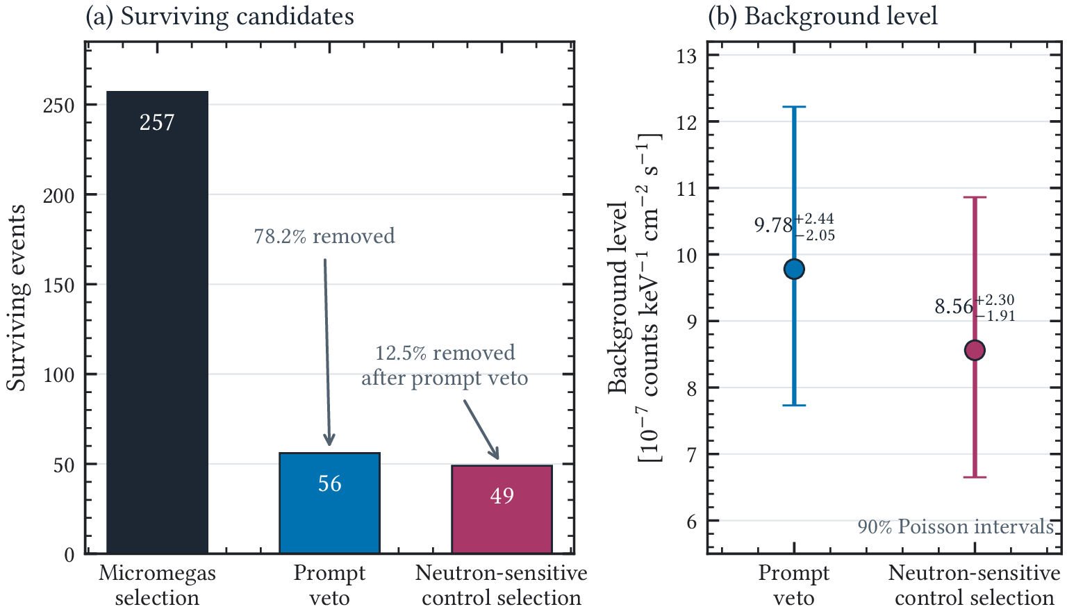
The IAXO-D0 prototype supplies the principal experimental result. In 52.1 d of surface data, the
prompt veto removes 201 of 257 Micromegas-selected events and the advanced selection removes a
further 7 of 56. The resulting background level is \((8.56^{+2.30}_{-1.91})\times 10^{-7}\) counts keV−1 cm−2 s−1 at 90% confidence, with
97.0% retention of the Micromegas-selected calibration sample. The additional rejection is
measured without identifying the rejected events individually as neutrons. These results support
further validation using the existing data and simulations. An absolute BabyIAXO prediction
additionally requires its xenon–neon response, optics, final geometry, and site-specific source
normalization.
Resumen
BabyIAXO es la etapa intermedia del International Axion Observatory, un programa
para buscar axiones solares mediante su conversión en rayos X en un campo magnético
intenso. Su operación prevista en superficie requiere detectores que rechacen el fondo
cósmico y conserven una señal débil de rayos X de energía keV. Esta tesis desarrolla
métodos de simulación, modelado de fondo y veto activo para los detectores Micromegas de
IAXO.
El trabajo amplía REST-for-Physics y su interfaz con Geant4, restG4, mediante
herramientas de generación de fuentes, geometrías, respuesta del detector y producción a gran
escala. Para IAXO-D1 con argón–isobutano, un inventario organiza los fondos cósmicos,
ambientales e intrínsecos bajo una selección común de sucesos reconstruidos. Se documentan los
primarios generados y los requisitos de normalización pendientes. Los clasificadores topológicos
muestran diferencias importantes entre simulación y datos; por ello, la selección de referencia no
les atribuye rechazo de fondo.
Los estudios de blindaje identifican las cascadas secundarias producidas por neutrones de alta
energía en el plomo como un mecanismo de fondo relevante. Motivan un veto multicapa de
centelleador plástico y cadmio que combina actividad rápida y capturas retardadas. Tres capas
ofrecen un compromiso entre identificación condicional y complejidad. Una eficiencia neutrónica
cuantitativa requiere validar la aceptación temporal, el quenching y las capturas. La activación se
evalúa por separado mediante simulaciones de producción y desintegración, sin aplicar rechazo
rápido a desintegraciones retardadas.
El principal resultado experimental procede de IAXO-D0. En 52.1 d de datos, el veto rápido
elimina 201 de 257 sucesos seleccionados por Micromegas; la selección avanzada elimina otros 7 de
los 56 restantes. El fondo resultante es \((8.56^{+2.30}_{-1.91})\times 10^{-7}\) counts keV−1 cm−2 s−1 al 90% de confianza, conservando el
97.0% de la muestra de calibración seleccionada por Micromegas. El rechazo adicional está medido,
sin identificar individualmente como neutrones los sucesos rechazados. Estos resultados permiten
avanzar con los datos disponibles y nuevas simulaciones. Una predicción absoluta para BabyIAXO
requiere además su respuesta en xenón–neón, óptica, geometría final y normalización de fuentes
en el emplazamiento.
The Standard Model of particle physics provides an exceptionally successful description of the
known elementary particles and their interactions. Nevertheless, several observations and
theoretical questions point to physics beyond this framework. Among them, the nature of dark
matter and the absence of observed \(\mathrm {CP}\) violation in the strong interaction remain two of the most
compelling open problems. The axion was originally proposed as a dynamical solution to the
strong \(\mathrm {CP}\) problem, but it also emerged as a well-motivated dark-matter candidate [1–7].
More generally, axion-like particles appear naturally in many extensions of the Standard
Model and can be searched for through their weak couplings to photons, electrons, and
nucleons [8–10].
Solar axion helioscopes exploit one of the most direct experimental signatures of
these particles. If axions are produced in the solar interior, they can traverse the Sun
and the interplanetary medium essentially unattenuated. Inside a strong transverse
laboratory magnetic field, a small fraction can convert coherently into X-ray photons. The
experimental task is therefore conceptually simple but technically demanding: point a
powerful magnet toward the Sun, focus any converted photons onto a small detector area,
and identify a possible excess of keV X-rays above an extremely low background [11,
12].
The International Axion Observatory (IAXO) is designed as the next major step in this
technique, building on the experience of previous helioscopes and especially on the CERN Axion
Solar Telescope (CAST) [13]. BabyIAXO is the intermediate stage of this program [14]. It is
intended to validate the main technologies required for IAXO while also operating as a competitive
helioscope in its own right. The March 2026 outdoor working baseline brings low-background
X-ray detection, solar tracking, and mechanical integration together in a surface environment [15].
Its detector development must therefore address cosmic-ray backgrounds under realistic operating
conditions.
This thesis focuses on the IAXO Micromegas detector program, spanning IAXO-D0,
IAXO-D1, and the separate BabyIAXO projection. Microbulk Micromegas detectors are well
suited to helioscope searches because they combine low intrinsic radioactivity, good
energy response in the keV range, topological discrimination, and compatibility with
compact shielding and focusing optics [16, 17]. However, the expected signal rate is
extremely small. The physics reach of the experiment therefore depends not only on detector
performance, but also on the reliability of the background model, the realism of the
detector-response simulation, and the effectiveness of the shielding and active veto
strategy.
The work presented here addresses these requirements from three connected directions. First, it
describes contributions to the software and simulation infrastructure used by the collaboration,
with particular emphasis on REST-for-Physics, its Geant4 interface restG4, and the
production workflows needed for large Monte Carlo campaigns. Second, it develops a
source-resolved background inventory for IAXO-D1 in argon–isobutane, combining radiopurity
information, environmental measurements, cosmic-ray models, and detector-response simulations.
A BabyIAXO prediction additionally requires its xenon–neon response, focusing optics,
final veto, and site-specific DESY source environment. Third, it studies the surface-level
cosmic-ray-induced background and the corresponding active veto system, including the
optimization of a multilayer plastic-scintillator and cadmium design, waveform-level veto
observables, construction and commissioning aspects, and comparison with experimental
data.
A central theme of the thesis is the transition from idealized background estimates to analysis
objects that can be compared with real detector data. The relevant question is not only whether a
simulated particle deposits energy in the detector volume, but whether the resulting event would
pass the same energy, topology, timing, and veto selections applied to the experimental data. For
this reason, the simulations are propagated through a detector-response chain whenever possible,
and the veto studies are expressed in terms of prompt signals, delayed activity, channel
multiplicity, and reconstructed observables. This approach is especially important for surface
operation, where muons, high-energy neutrons, and secondary particles produced in the shielding
can generate backgrounds that are not adequately described by passive shielding arguments
alone [17].
Contribution
Chapter
Scope
and
evidence
Simulation
infrastructure
4
Source
generation,
versioned
geometry,
transport,
and
common
reconstruction
of
detector
observables.
Shielding
and
active
veto
5
Mechanism-based
surface-neutron
study,
conditional
multilayer
comparisons,
and
timing
and
multiplicity
observables.
Experimental
veto
analysis
5
Measured
prompt
and
additional
delayed/multiplicity
rejection
in
IAXO-D0;
no
neutron
identity
is
assigned
to
the
rejected
events.
Background
inventory
6
Source-specific
counts,
yields,
and
normalization
requirements
for
IAXO-D1;
missing
or
incompatible
components
remain
explicit.
Activation
and
response
validation
6
Production
and
decay-response
simulations,
an
incident-photon
efficiency
ledger,
and
tests
of
simulation-to-data
transfer.
Table 1:
Main
contributions
of
the
thesis.
The
software
and
analysis
developments
are
evaluated
through
the
physical
studies
summarized
in
the
final
column.
The structure of the thesis follows this logic. Chapter 1 introduces the axion and
axion-like-particle motivation, the strong \(\mathrm {CP}\) problem, and the main experimental approaches used in
axion searches. Chapter 2 describes the IAXO program, the helioscope figure of merit, the role of
BabyIAXO, and the experimental context in which the detector work is carried out. Chapter 3
presents the Micromegas detector technology, the IAXO-D0 and IAXO-D1 detector prototypes and
their relation to BabyIAXO, and the associated gas, high-voltage, slow-control, data-acquisition,
and calibration systems. Chapter 4 describes the computational framework used in the thesis,
including ROOT, REST-for-Physics, restG4, data production, visualization,
and related software developments. Chapter 5 studies the shielding and veto system,
with emphasis on cosmic-ray-induced backgrounds, passive-shielding limitations, the
active scintillator–cadmium veto concept, and the comparison between simulations and
prototype data. Chapter 6 presents the IAXO-D1 argon source-response model, including
intrinsic, environmental, cosmic, and neutron-induced activation contributions, the
common selection, the generated-primary denominators, and the unresolved inputs needed
for an absolute total. The conclusions assess the established results and prioritize the
response and source-validation studies needed for IAXO-D1 and the subsequent BabyIAXO
projection.
Chapter 1 Axions and Axion-Like Particles
1.1 Motivation and Scope
The QCD axion is a hypothetical pseudoscalar particle predicted by the most widely studied
dynamical solution to the strong \(\mathrm {CP}\) problem. Its small mass and weak interactions also make it a
viable cold-dark-matter candidate over broad, cosmology-dependent regions of parameter
space. Axion-like particles (ALPs) share similar interactions but need not solve the strong
\(\mathrm {CP}\) problem and do not obey the QCD relation between mass and couplings. Both classes of
particles arise in extensions of the Standard Model and motivate a diverse experimental
program [8–10].
This chapter introduces only the physics required to place solar helioscopes in that program. It
summarizes the strong \(\mathrm {CP}\) problem, the Peccei–Quinn mechanism, the interactions most relevant to
experiments, and the principal cosmological and astrophysical motivations. The emphasis is on the
axion-photon coupling because it governs both solar production through the Primakoff process and
coherent conversion in a laboratory magnetic field. The corresponding solar spectra, conversion
probability, coherence conditions, buffer-gas operation, and helioscope figure of merit are
developed in the next chapter.
The observable solar signal is the product of the axion flux, the probability of conversion in the
magnet, and the detector acceptance. Even a large incident flux can therefore produce only a few
detected X rays. For IAXO and BabyIAXO, the detector must combine efficient, stable
operation in the 1–10 keV region with strong rejection of instrumental and environmental
backgrounds.
1.2 The Strong CP Problem and the QCD Axion
The most general quantum chromodynamics (QCD) Lagrangian contains a term that violates parity
and \(\mathrm {CP}\),
Here, \(G_{\mu \nu }^{a}\) is the gluon field-strength tensor, \(\widetilde {G}^{a,\mu \nu }=\varepsilon ^{\mu \nu \lambda \rho }G_{\lambda \rho }^{a}/2\) is its dual, \(\alpha _{\mathrm {s}}\) is the strong coupling, and \(M_q\) is the quark
mass matrix. The physical angle \(\bar {\theta }\) combines the bare QCD angle with a phase from the
quark masses. This source of strong-interaction \(\mathrm {CP}\) violation is distinct from the observed
Cabibbo–Kobayashi–Maskawa phase in the weak sector. Although setting \(\bar {\theta }\) to zero is compatible
with observation, the Standard Model contains no symmetry that requires this value once the
quark masses are complex. The difficulty is therefore not an inconsistency of QCD but the
unexplained hierarchy between the allowed natural scale of the parameter and its experimental
upper bound.
The neutron electric dipole moment (nEDM) provides the most direct constraint on \(\bar {\theta }\). The 2020
measurement, which remained the most stringent direct limit as of September 2026,
gives [18]
Hadronic calculations place \(d_n/\bar {\theta }\) at order \(10^{-16}\,e\,\si {cm}\), with a coefficient that depends on the calculation
method [10, 19, 20]. Equation 1.2 therefore requires \( |\bar {\theta }|\lesssim \mathcal {O}(10^{-10}) \). Explaining why a dimensionless parameter
that could naturally be of order unity is so small constitutes the strong \(\mathrm {CP}\) problem. Other proposed
solutions impose fundamental \(\mathrm {CP}\) symmetry or modify the light-quark sector, but they require
additional model structure. The Peccei–Quinn (PQ) mechanism is particularly economical because
the same dynamics that removes \(\bar {\theta }\) predicts a particle that can be searched for experimentally [8,
10].
The PQ mechanism promotes this fixed angle to a dynamical degree of freedom [1, 2]. A global
\(U(1)_{\mathrm {PQ}}\) symmetry is spontaneously broken at a scale \(f_a\), producing a pseudo-Nambu–Goldstone field \(a(x)\). Its
QCD anomaly gives the effective interaction
Nonperturbative QCD generates a potential whose minimum satisfies \(\langle a\rangle /f_a=\bar {\theta }\). The effective strong
\(\mathrm {CP}\) angle then vanishes dynamically, while fluctuations about the minimum constitute the axion [3,
4]. This sign convention is consistent with Eq. 1.1; reversing the definition of \(a\) would change both
axion signs without changing observables.
The same QCD dynamics fixes the axion mass through the topological susceptibility. Modern
chiral and lattice calculations give [21, 22]
Consequently, a larger PQ scale produces a lighter and more weakly coupled axion. Axions
with \(f_a\) near the electroweak scale were excluded by laboratory measurements, whereas
invisible-axion models with \(f_a\gg v_{\mathrm {EW}}\) remain viable. This inverse relation between mass, interaction
strength, and the symmetry-breaking scale explains why viable axions are challenging to detect
and why large magnetic volumes, long exposures, and low-background detectors are
required.
1.3 Interactions and Axion-Like Particles
The gluonic interaction in Eq. 1.3 is essential to the solution of the strong \(\mathrm {CP}\) problem, but couplings
to photons, electrons, and nucleons depend on the ultraviolet realization of the PQ symmetry. The
photon interaction can be written as
Here, \(E/N\) is the electromagnetic-to-color anomaly ratio of the PQ current, while \(F_{\mu \nu }\) and \(\widetilde {F}^{\mu \nu }\) are
the electromagnetic field-strength tensor and its dual. The second term includes the
model-independent contribution from mixing with neutral mesons [10, 21]. For QCD axions,
Eqs. 1.4 and 1.5 produce an approximately linear band in the \((m_a,g_{a\gamma })\) plane rather than two independent
parameters.
KSVZ and DFSZ constructions provide common reference models [23–26]. In the simplest
KSVZ model, the anomaly is generated by a new heavy quark; an electrically neutral heavy quark
gives \(E/N=0\). In DFSZ models, Standard Model fermions couple through an extended Higgs sector, with \(E/N=8/3\)
in the commonly used benchmark. These values are useful reference lines but do not encompass all
viable QCD-axion couplings. The electron coupling is defined here by \begin{equation} \mathcal {L}_{ae}=-i g_{ae}a\bar {e}\gamma _5 e, \qquad g_{ae}=\frac {C_e m_e}{f_a}. \label {eq:axion-electron-coupling} \end{equation} Thus \(g_{ae}\) is dimensionless,
whereas \(g_{a\gamma }\) has dimensions of inverse energy. The coefficient \(C_e\) conventionally appears in the
derivative interaction \(C_e(\partial _\mu a)\bar {e}\gamma ^\mu \gamma _5e/(2f_a)\). The electron equations of motion relate it to the pseudoscalar form
above; a change of operator basis must also account consistently for the anomalous
photon term [8, 27]. Electron and nucleon couplings control additional solar production
channels, stellar energy loss, and searches through interactions with matter. Their model
dependence is kept explicit when reporting limits on production–detection coupling
products.
The interaction in Eq. 1.5 permits several physically distinct processes. In the microscopic
Coulomb field of a charged particle, photon–axion scattering is the Primakoff process. In a
macroscopic transverse magnetic field, axion and photon states instead undergo coherent mixing,
which can be described as oscillation between the two states. A material medium changes the
photon dispersion relation and can restore phase matching; it does not simply supply a second real
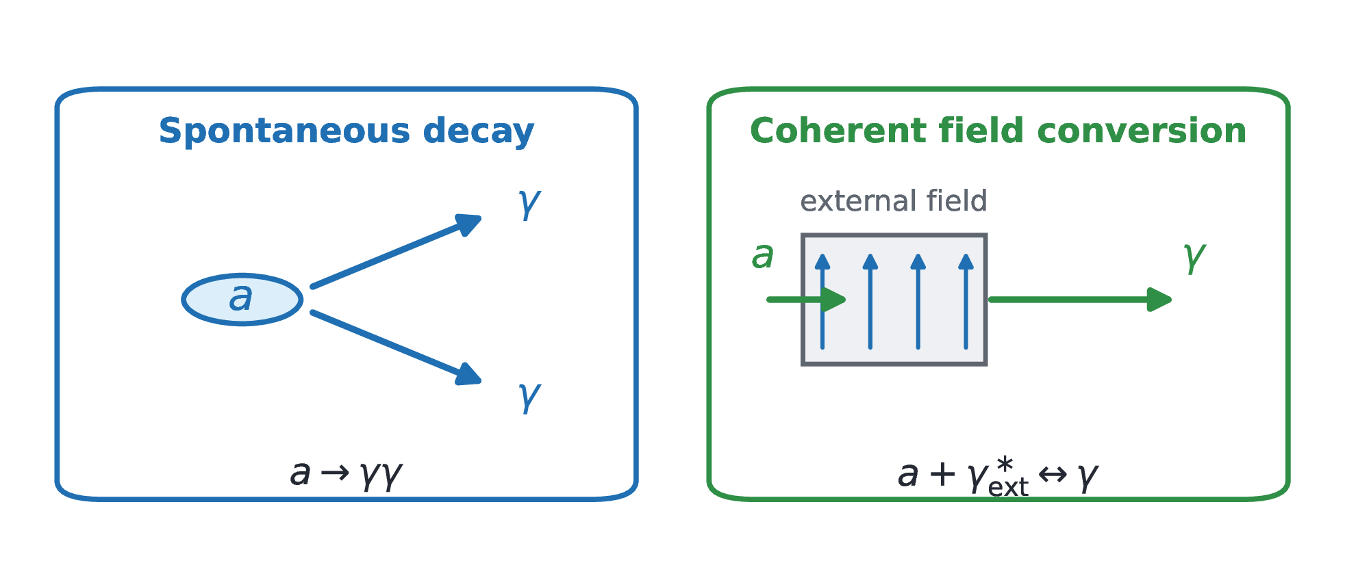
photon. Spontaneous \(a\rightarrow \gamma \gamma \) decay is also allowed. In natural units, \(\hbar =c=1\), its decay width and lifetime are
\begin{equation} \Gamma _{a\rightarrow \gamma \gamma } = \frac {g_{a\gamma }^{2}m_a^{3}}{64\pi }, \qquad \tau _{a\rightarrow \gamma \gamma } = \Gamma _{a\rightarrow \gamma \gamma }^{-1}. \label {eq:axion-two-photon-lifetime} \end{equation}
The strong inverse dependence on both mass and coupling makes this decay extraordinarily
slow for the light, weakly coupled particles relevant to helioscopes. For example, \(m_a=1\,\mathrm{meV}\) and \(g_{a\gamma }=1\times10^{-14}\,\mathrm{GeV}^{-1}\) give \(\tau _{a\rightarrow \gamma \gamma }\simeq 4\times10^{34}\,\mathrm{yr}\). The
decay is therefore negligible on laboratory, solar-system, and cosmological timescales for this
benchmark; coherent conversion in an external field is the experimentally relevant process [10, 28,
29].
Figure 1.1: Two consequences of the axion-photon interaction. A free axion can decay into
two photons, whereas a transverse macroscopic magnetic field produces coherent
axion-photon mixing. Solar helioscopes use the latter process to convert solar axions into X
rays; a medium may modify the photon dispersion relation and hence the phase matching.
An ALP is a light pseudoscalar with axion-like interactions but without the strict QCD relation
between mass and couplings. Such fields can result from approximate global symmetries, hidden
sectors, or string compactifications, and they need not solve the strong \(\mathrm {CP}\) problem [30–33].
Experiments therefore report both QCD-axion interpretations, represented by a model band, and
more general ALP limits in which \(m_a\) and \(g_{a\gamma }\) are independent. This broader interpretation is useful for
helioscopes because the same detector can test a QCD axion and any sufficiently light ALP
produced by the same solar processes. Only the mapping from the measured coupling limit to an
underlying particle model changes.
1.4 Cosmological and Astrophysical Context
Axions can form cold dark matter through nonthermal production. The canonical mechanism is
vacuum misalignment: after PQ symmetry breaking, the axion field is generally displaced from the
minimum of its potential. When the expansion rate falls to approximately \(3H(T_{\mathrm {osc}})\simeq m_a(T_{\mathrm {osc}})\), the field begins
coherent oscillations whose energy density subsequently redshifts approximately as nonrelativistic
matter [9, 34].
The predicted abundance depends strongly on the cosmological history. If PQ symmetry
breaking occurs before inflation and is not restored afterward, the observable Universe inherits one
initial misalignment angle, and isocurvature constraints connect the model to the scale of inflation.
If it occurs after inflation, different regions begin with different angles, while axion strings and
domain walls can contribute to the abundance. For this reason, cosmology does not select one
unique axion mass or require axions to constitute all dark matter. Haloscope interpretations also
depend on the assumed local halo density and velocity distribution, whereas helioscopes do not
depend on the cosmological axion abundance. The distinction is important when comparing
exclusion plots: a haloscope limit can weaken if axions are only a subcomponent of the halo, while
a helioscope limit continues to constrain the relevant solar-production and photon-conversion
couplings.
Thermally produced axions provide a separate cosmological probe. If sufficiently light and
long-lived, they contribute a hot relic component that affects the cosmic microwave background
and the growth of large-scale structure. The resulting constraints depend on the thermal history,
the relevant axion couplings, and the cosmological data combination, so they are best
stated as model-dependent limits rather than as a single universal mass bound [10,
35].
Stellar environments constrain weakly coupled particles because axions can escape and carry
away energy. The Primakoff process in horizontal-branch stars and the Sun probes \(g_{a\gamma }\), while red
giants, white dwarfs, supernovae, and neutron stars test complementary electron and
nucleon couplings [35, 36]. These bounds follow from agreement between observed stellar
populations or evolution and models that include an additional energy-loss channel.
Their reliability depends on the object and observable, so limits from several systems
should not be treated as statistically interchangeable. Some stellar observations have been
interpreted as possible cooling anomalies, but their present significance does not constitute
evidence for axions. They instead define motivated targets that should be tested with
controlled experiments. Solar helioscopes are especially valuable in this respect because
they search directly for particles emitted by the Sun without requiring axions to be
Galactic dark matter. Their interpretation still relies on solar modeling, but the solar
interior is constrained by helioseismology and neutrino measurements, and the signal
can be modulated experimentally by alternating between tracking and nontracking
periods.
1.5 Search Landscape and the Role of Helioscopes
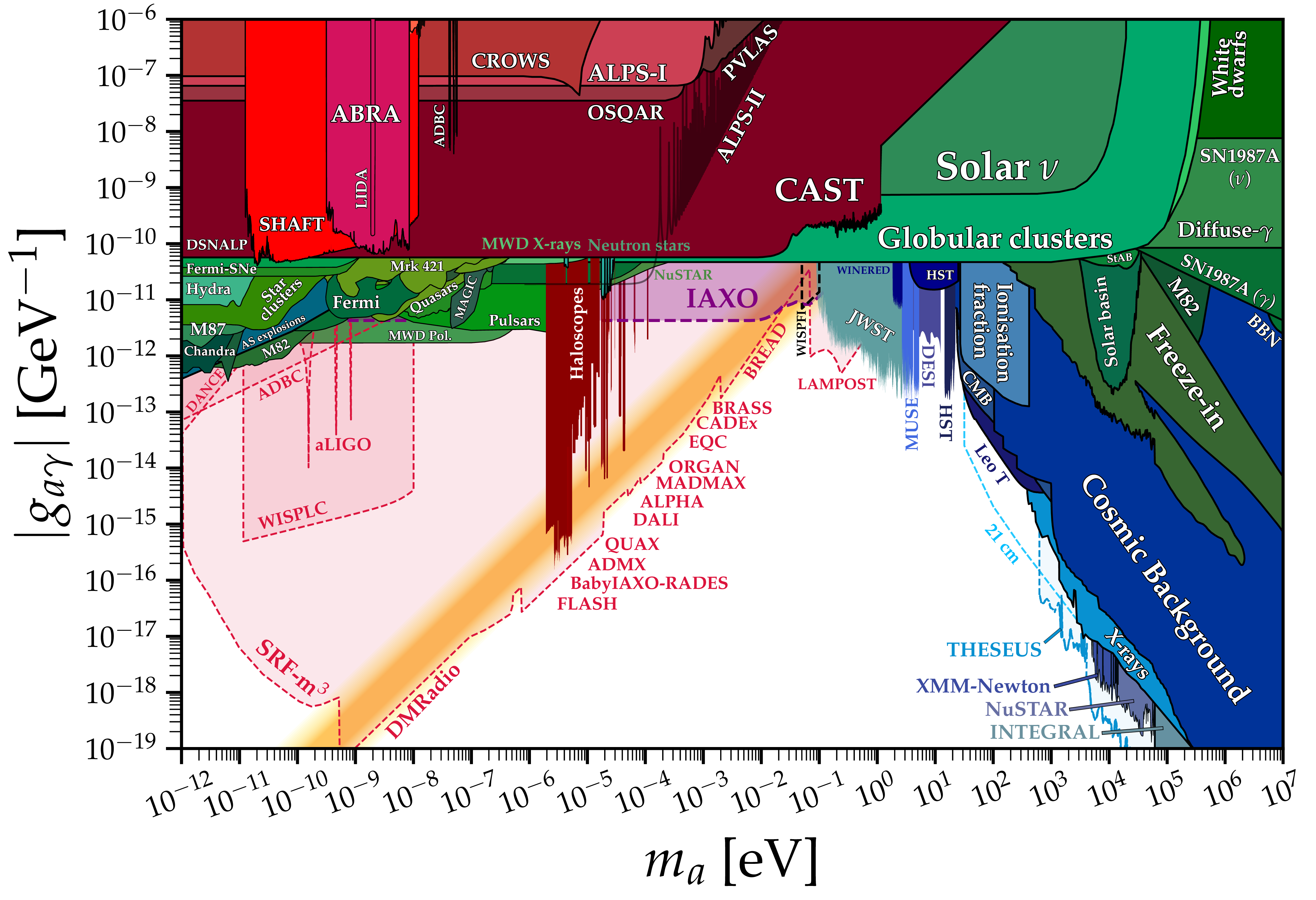
Axion experiments exploit complementary assumptions and interactions [10, 37, 38]. Figure 1.2
gives a selective orientation to the principal photon-coupling searches relevant here rather than an
exhaustive compilation.
Figure 1.2: Selective overview of the axion-photon parameter space. The digitized CAST,
globular-cluster, ALPS I, and haloscope boundaries and the design projections use the
checksum-verified AxionLimits snapshot [39]; the underlying CAST, stellar, and ALPS I
results are given in Refs. [40–42]. The added ALPS II segment shows its reported 95%
low-mass limit from the 2024 science campaign, only for \(m_a\lesssim 0.1\,\mathrm{meV}\) [43]. Solid boundaries denote
observed limits; unfilled dashed curves denote design projections, including the separate
ALPS II design target. The hatched model band and KSVZ/DFSZ lines use the central
constants in Eqs. 1.4 and 1.5. Haloscope limits are shown for a local dark-matter density of
\(\rho _{\mathrm {DM}}=0.45\,\si {GeV\,cm^{-3}}\) and therefore assume a Galactic axion population. Stellar and helioscope limits do not
require axions to constitute the local dark matter.
The boundaries in Figure 1.2 have different statistical and physical interpretations. CAST
reports a 95% Bayesian upper limit with a prior uniform in nonnegative \(g_{a\gamma }^{4}\), using a solar
Primakoff flux [40]. The globular-cluster bound uses the ratio of asymptotic-giant-branch to
horizontal-branch populations and depends on the treatment of convective mixing [41]. The
haloscope curve is an envelope of searches with distinct mass coverage and analysis assumptions,
rather than a joint likelihood [10, 39]. The digitized curves are approximate representations of
those results; in particular, the published low-mass CAST limit is \(5.8\times10^{-11}\,\mathrm{GeV}^{-1}\). The BabyIAXO and IAXO curves
retain their published design assumptions [13, 14].
Haloscopes use a magnetic field and a resonant or broadband electromagnetic structure to
convert nonrelativistic Galactic axions into photons. They have reached benchmark QCD-axion
sensitivity in selected mass regions, but their interpretation assumes a local dark-matter
population. The broader program includes microwave cavities, dielectric structures,
lumped-element circuits, plasma concepts, and quantum sensors. Because resonant instruments
cover a limited frequency interval at one time, much of this program proceeds through systematic
scans across axion mass.
Light-shining-through-wall experiments generate ALPs from a laser in one magnetic region,
block the photons, and search for regenerated photons after a second magnetic region. This is a
laboratory-only test that is independent of astrophysical-source and cosmological-abundance
assumptions, although its production-and-regeneration probability scales as \(g_{a\gamma }^{4}\). The ALPS II
campaign of February–May 2024 found no signal and set a 95% upper limit of \(\lvert g_{a\gamma }\rvert <1.5\times10^{-9}\,\mathrm{GeV}^{-1}\) for pseudoscalar
masses below approximately \(0.1\,\mathrm{meV}\) [43]. Its projected reach assumes the upgraded optical configuration
and is shown separately from this measurement.
Other searches target axion interactions with matter. Low-threshold detectors can
search for axion absorption through electron couplings. CASPEr uses nuclear magnetic
resonance and spin-precession observables to probe oscillating axion-induced moments and
fields, whereas ARIADNE searches for an axion-mediated spin-dependent force [37, 44].
Together, these approaches retain sensitivity when the photon coupling is suppressed. No
single method covers the full parameter space: resonant dark-matter searches provide
high sensitivity over narrow mass intervals, laboratory production minimizes source
assumptions, and helioscopes combine broad mass acceptance with sensitivity to solar
production.
Helioscopes search for relativistic axions continuously produced in the Sun, using coherent
conversion in a transverse laboratory magnetic field. The observable is a tracking-correlated excess
of focused X rays, independent of the local dark-matter density. Optics reduce the detector area
collecting background while preserving the magnet aperture, linking the three principal elements
of the IAXO design [45]. The next chapter develops the solar spectra, conversion probability, and
exposure requirements for this search.
Chapter 2 The Helioscope Technique and the IAXO Program
Introduction
Solar helioscopes combine a well-characterized astrophysical source with magnetic conversion and
a tracking-correlated X-ray signal. This chapter develops the signal yield and statistical sensitivity,
then follows the progression from CAST to the International Axion Observatory (IAXO) and its
intermediate stage, BabyIAXO [13, 14, 46]. The connection to the present work is the
detector-background requirement: a larger magnetic aperture is useful only if the optics and
detector retain the converted photons while suppressing the background collected with
them. Published design projections, the March 2026 engineering and site studies, and the
subsequent funding milestone are distinguished below; the project-status cutoff is September
2026.
2.1 The Helioscope Technique
2.1.1 Solar Axions
Solar axions are produced in the hot, dense plasma of the Sun through several processes. The best
known is Primakoff conversion, in which thermal photons convert into axions in the
electromagnetic fields of charged plasma constituents. Additional contributions arise from
processes involving the axion–electron coupling: atomic axio-recombination and axio-deexcitation,
electron–ion and electron–electron bremsstrahlung, and Compton-like scattering. These processes
are commonly grouped as the ABC channels [27].
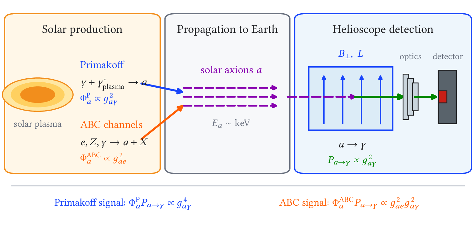
Figure 2.1: Schematic production and detection chain for solar axions in a helioscope.
Primakoff production in the solar plasma is controlled by \(g_{a\gamma }\), whereas ABC production is
controlled by \(g_{ae}\). Detection in the magnet occurs through inverse Primakoff conversion and
therefore depends on \(g_{a\gamma }\).
The coupling dependence follows directly from this chain. For Primakoff solar axions, both
production in the Sun and conversion in the laboratory depend on \(g_{a\gamma }\), so the expected signal rate
scales as \(g_{a\gamma }^{4}\). For ABC solar axions, production depends on \(g_{ae}\), whereas detection still requires
axion–photon conversion, so the signal rate scales as \(g_{ae}^{2}g_{a\gamma }^{2}\). Primakoff data therefore constrain \(\lvert g_{a\gamma }\rvert \), whereas
ABC data constrain the product \(\lvert g_{ae}g_{a\gamma }\rvert \). Separating the two couplings requires an additional model
assumption or an independent constraint.
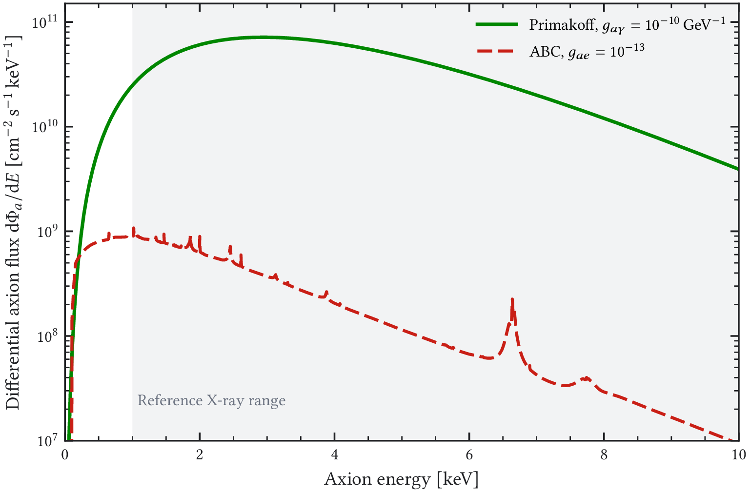
Figure 2.2: Disk-integrated differential solar axion flux at Earth for two benchmark
couplings. The Primakoff spectrum uses the archived SolarAxionFlux v0.9 tabulation, dated
March 21, 2022, for \(g_{a\gamma }=1\times10^{-10}\,\mathrm{GeV}^{-1}\) [47]; the ABC spectrum uses the tabulation of Redondo for \(g_{ae}=10^{-13}\) [27]. Both
spectra are shown on the same logarithmic vertical scale, preserving their relative
normalization.
Figure 2.2 shows the corresponding spectral components in the energy range relevant to
helioscope searches. The Primakoff spectrum peaks at a few kiloelectronvolts, within the reference
Micromegas analysis band of approximately \(1\text{--}10\,\mathrm{keV}\). The electron-coupling channels produce a softer
component, motivating focal-plane detectors with sub-kiloelectronvolt thresholds, such as GridPix
and cryogenic sensors. Integrating the archived Primakoff table over \(0.01\text{--}20\,\mathrm{keV}\) gives \(\Phi _a=3.46\times10^{11}\,\mathrm{cm}^{-2}\,\mathrm{s}^{-1}\) and a mean energy of \(4.14\,\mathrm{keV}\)
at the stated coupling. Its preserved header specifies the generator version and couplings but not
the solar-model or opacity configuration, so no particular solar model is assigned to this tabulation.
It is used here to illustrate the spectrum; a quantitative signal prediction must retain the
model inputs and their uncertainties. The comparison of solar models in Ref. [47] finds a
Primakoff-flux systematic difference of approximately 5%, in addition to uncertainty within each
model.
The continuum channels shown here are appropriate to the few-kiloelectronvolt Micromegas
study. At lower thresholds, longitudinal-plasmon conversion in solar magnetic fields
can provide an additional \(g_{a\gamma }\)-dependent source and may dominate below approximately \(200\,\mathrm{eV}\),
depending on the solar-field profile [48]. The benefit of sub-kiloelectronvolt detectors
therefore extends beyond the ABC spectrum, while requiring a broader solar-source
model.
2.1.2 Axion–Photon Conversion in a Helioscope
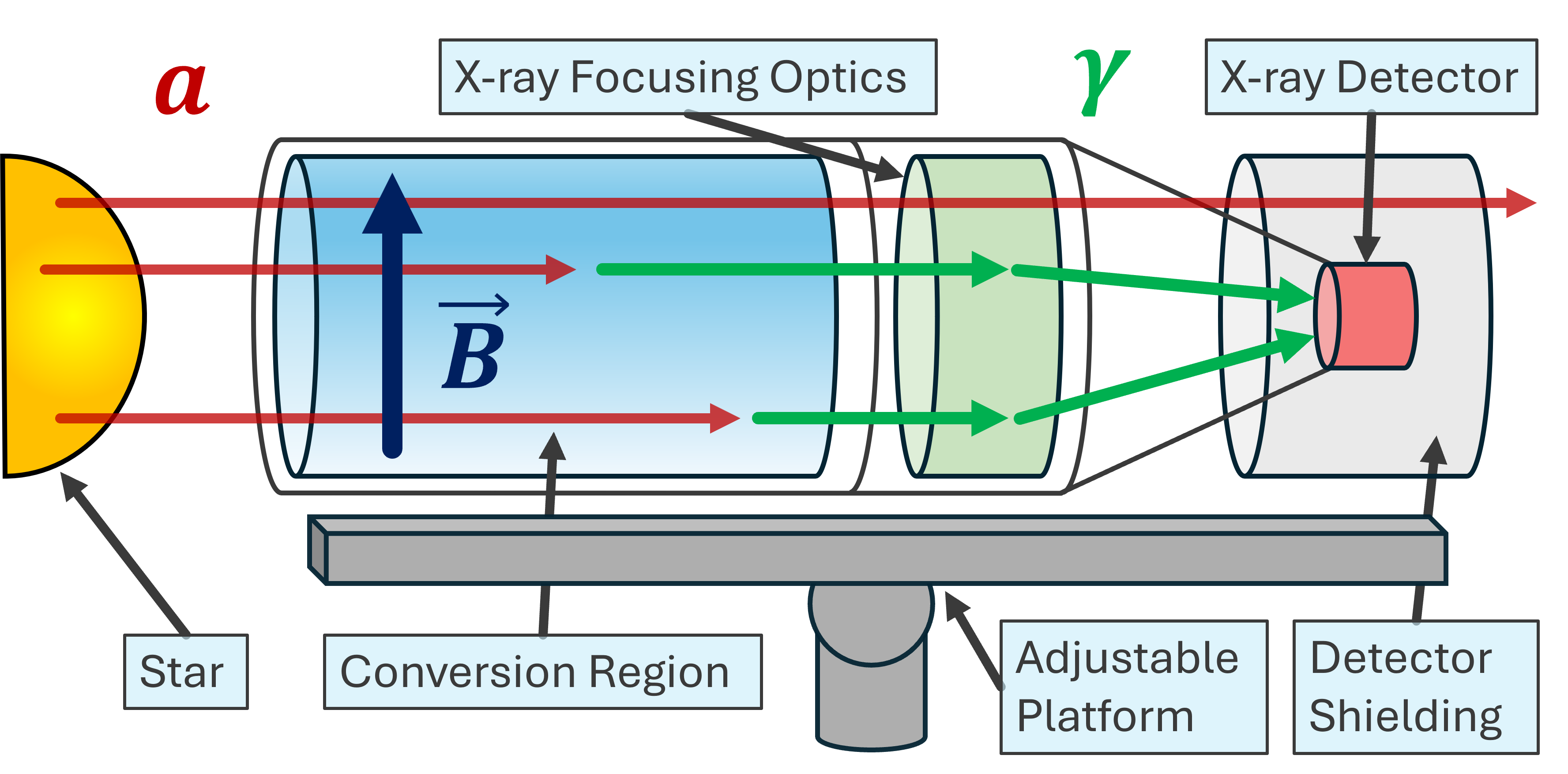
Figure 2.3: Conceptual diagram of a helioscope. Solar axions enter a magnetic conversion
region mounted on a mobile platform that tracks the Sun. The converted X-ray photons are
focused by X-ray optics onto a low-background detector.
The operating principle is illustrated in Figure 2.3. Solar axions traverse a strong transverse
magnetic field and can convert into X-ray photons through the inverse Primakoff effect.
Grazing-incidence optics focus those photons onto a detector optimized for the relevant energy
range, while a mobile platform follows the Sun during the daily tracking window.
In natural units, \(\hbar =c=1\), the conversion probability for a homogeneous transverse magnetic field \(B_\perp \) of
length \(L\), neglecting photon absorption, is \begin{equation} P_{a \rightarrow \gamma }(L) = {\left (\frac {g_{a\gamma } B_\perp L}{2}\right )}^{2} \mathcal {F}(qL). \label {eq:helioscope-conversion-probability} \end{equation}
The coherence factor is \begin{equation} \mathcal {F}(qL) = {\left (\frac {2}{qL}\right )}^{2} \sin ^{2}\left (\frac {qL}{2}\right ). \label {eq:helioscope-coherence-factor} \end{equation}
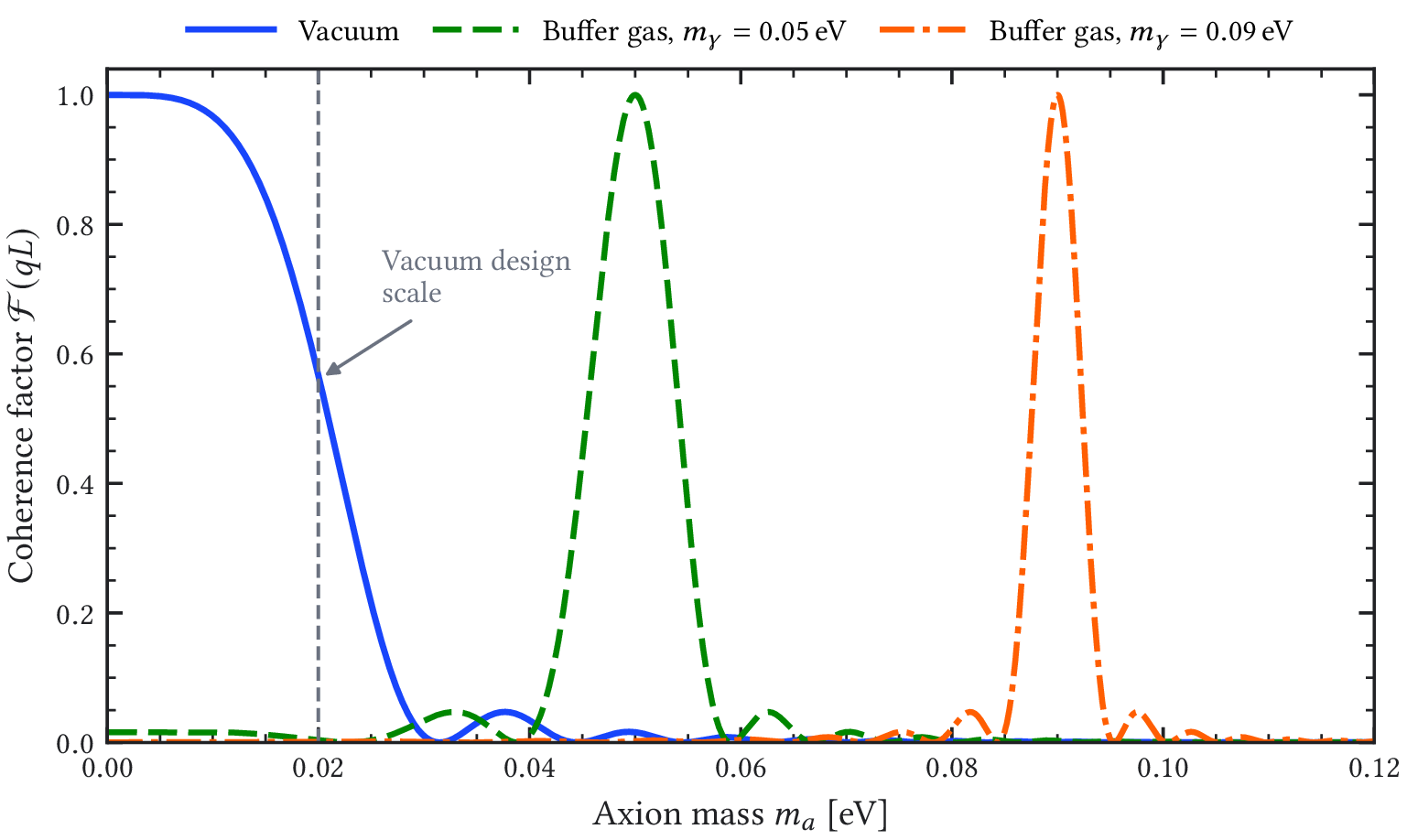
In vacuum, \(q \simeq m_a^2/(2E)\) for a relativistic axion of energy \(E\). The coherent regime corresponds to \(qL \ll 1\), for which \(\mathcal {F} \simeq 1\)
and the conversion probability grows as \(B_\perp ^2L^2\).
At larger axion masses, the axion–photon momentum mismatch suppresses conversion. A
buffer gas gives the photon an effective mass \(m_\gamma \), changing the mismatch to \(q \simeq \lvert m_a^2-m_\gamma ^2\rvert /(2E)\) and restoring coherence
over a narrow mass interval. Equations 2.1 and 2.2 remain the negligible-absorption expression
after this substitution; a realistic gas scan must also include photon absorption and density
gradients [49–51]. Vacuum is recovered by setting \(m_\gamma =0\).
For X-ray energies well above the atomic resonances of a low-\(Z\) gas, the effective mass is its
plasma frequency, \begin{equation} m_\gamma ^2 = \omega _{\mathrm {pl}}^2 = \frac {4\pi \alpha n_e}{m_e}. \label {eq:buffer-gas-photon-mass} \end{equation}
Here, \(n_e\) is the electron density and \(m_e\) is the electron mass. At fixed temperature and composition, \(n_e\)
is proportional to the gas pressure, so each pressure setting selects a different resonant value \(m_a\simeq m_\gamma \). The
coherent interval at one setting is narrow; an extended mass range is therefore covered by
increasing the pressure in overlapping steps rather than by operating at one fixed pressure. This
relation between gas density, effective photon mass, and coherence is the basis of the CAST
buffer-gas campaigns described below.
Figure 2.4: Coherence factor for \(E=4\,\mathrm{keV}\) axions in a \(L=10\,\mathrm{m}\) homogeneous magnetic field. Vacuum
conversion remains coherent only at sufficiently low mass, whereas a buffer gas restores
coherence around the mass for which \(m_a \simeq m_\gamma \). The illustrative gas curves neglect photon
absorption and density gradients.
For one detection line, the expected differential event yield can be written schematically as
\begin{equation} \frac {\mathrm {d}N_\gamma }{\mathrm {d}E} = \frac {\mathrm {d}\Phi _a}{\mathrm {d}E} P_{a\rightarrow \gamma }(E) A\,\epsilon _o(E)\,\epsilon _d(E)\,\epsilon _t\,t. \label {eq:helioscope-detected-spectrum} \end{equation}
Here, \(A\) is the instrumented aperture, \(\epsilon _o\) and \(\epsilon _d\) are the optics and detector efficiencies, \(\epsilon _t\) is the
tracking fraction, and \(t\) is the elapsed data-taking time. For a selected focal region, \(\epsilon _o\) includes the
fraction of the solar image retained within it. For multiple detection lines, the predicted spectra are
summed with their line-specific fields, apertures, and efficiencies. This expression connects the
solar spectra and conversion probability to the experimental sensitivity parameters discussed
next.
2.1.3 Experimental Figure of Merit
In the background-dominated regime, the principal design dependencies are summarized by the
helioscope figure of merit (FOM) [13, 46]: \begin{equation} f = f_M f_{DO} f_T. \label {eq:helioscope-fom} \end{equation}
Its components are \begin{equation} f_M = B_{\mathrm {eff}}^2 L^2 A, \qquad f_{DO} = \frac {\epsilon _d \epsilon _o}{\sqrt {ba}}, \qquad f_T = \sqrt {\epsilon _t t}. \label {eq:helioscope-fom-components} \end{equation}
Here \(A\) is the total instrumented aperture and \(B_{\mathrm {eff}}\) is the corresponding aperture-weighted
effective transverse field; for a uniform field, \(B_{\mathrm {eff}}=B_\perp \). For a nonuniform magnet, \(B_{\mathrm {eff}}^2L^2A\) denotes the field
integral \(\int _A\lvert \int _0^L \mathbf {B}_\perp \,\mathrm {d}\ell \rvert ^2\mathrm {d}A\) in the coherent limit. The detector–optics term contains the detector efficiency \(\epsilon _d\),
optics throughput \(\epsilon _o\), areal detector background level \(b\), and selected focal-region area \(a\).
The latter includes the optics point-spread function and the finite angular extent of the
solar source. The tracking term contains the tracking fraction \(\epsilon _t\) and total elapsed time
\(t\).
This decomposition shows why a next-generation helioscope requires more than a strong
magnet. The magnetic term increases with aperture, field strength, and length; the detector–optics
term increases with efficiency and decreases with the selected area and background level; and the
tracking term favors long daily exposure. Because the Primakoff signal scales as \(g_{a\gamma }^{4}\), the projected
coupling reach scales approximately as \(\lvert g_{a\gamma }\rvert \propto f^{-1/4}\).
2.1.4 Sensitivity with Few Background Events
The figure of merit assumes coherent conversion and enough background counts for a Gaussian
approximation; its original derivation uses approximately ten or more expected background events
as a guide [46]. The lowest IAXO background targets can fall below this regime. For uniform
background in an energy interval \(\Delta E\) and total focal area \(a\), \begin{equation} \mu _b=b\,a\,\Delta E\,T, \qquad T=\epsilon _t t, \label {eq:helioscope-expected-background} \end{equation} where \(T\) is the effective tracking
exposure. Combining the full-IAXO targets in Table 2.1 with an illustrative \(2\text{--}7\,\mathrm{keV}\) window
and \(3\,\mathrm{yr}\) of elapsed operation gives \(\mu _b=2.84\) for \(\epsilon _t=0.5\). If three years instead denotes effective tracking
exposure, the expectation is \(5.68\) events. These are alternative exposure definitions, not an
uncertainty interval. The three-year run duration is drawn from the conceptual-design
study [14]; the calculation does not reproduce its spectral acceptance or gas-scan exposure
allocation.
For a Primakoff search at a fixed trial axion mass, a suitable starting point is the Poisson
likelihood \begin{equation} \mathcal {L}(g_{a\gamma },\boldsymbol {\nu })= \prod _{\ell ,k}\operatorname {Pois}\!\left [ n_{\ell k}\,\middle |\, \left (\frac {g_{a\gamma }}{g_0}\right )^4 S_{\ell k}(\boldsymbol {\nu })+B_{\ell k}(\boldsymbol {\nu }) \right ]\mathcal {L}_{\mathrm {aux}}(\boldsymbol {\nu }). \label {eq:helioscope-poisson-likelihood} \end{equation} Here \(\ell \) identifies a detection line and observing condition, including the gas density, and \(k\)
identifies a bin in reconstructed energy and focal position. The signal \(S_{\ell k}\) at a reference coupling \(g_0\) is
obtained by folding the solar flux and magnetic conversion probability with the line-specific optics
and detector response. The background expectation is \(B_{\ell k}\); \(\mathcal {L}_{\mathrm {aux}}\) represents off-Sun measurements,
calibrations, and finite-simulation constraints on nuisance parameters \(\boldsymbol {\nu }\). This construction preserves
energy migration, focal containment, and selection losses instead of compressing them into one
constant efficiency.
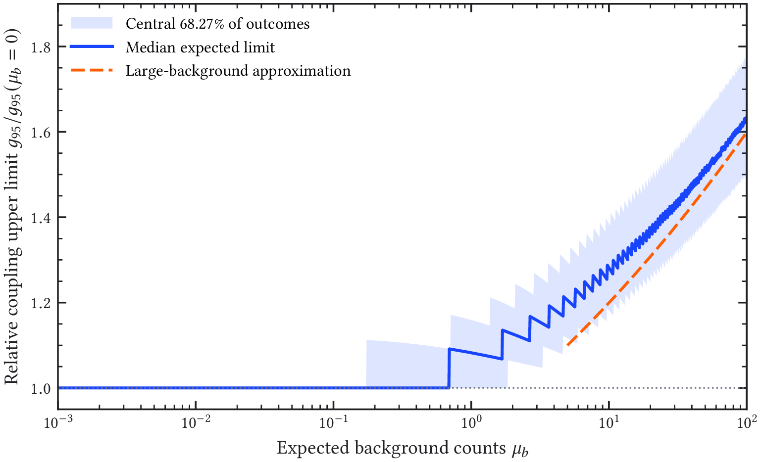
Figure 2.5 isolates the statistical effect using a single counting region with a known
background mean \(\mu _b\). For a signal mean \(s\geq 0\), a prior uniform in \(s\), and \(n\) observed events, the 95% Bayesian
upper bound satisfies \begin{equation} \frac {\displaystyle \int _0^{s_{95}}(s+\mu _b)^n e^{-(s+\mu _b)}\,\mathrm {d}s} {\displaystyle \int _0^\infty (s+\mu _b)^n e^{-(s+\mu _b)}\,\mathrm {d}s}=0.95. \label {eq:helioscope-counting-upper-limit} \end{equation} The prior is uniform in \(g_{a\gamma }^{4}\) for a fixed Primakoff response, as in the CAST
analysis [40]; other interval constructions need not give identical bounds [52]. At zero observed
events, \(s_{95}=-\ln (0.05)=3.00\). Expected sensitivity is evaluated over \(n\sim \operatorname {Pois}(\mu _b)\), rather than by setting an observed count equal to a
possibly noninteger mean. For the illustrative \(\mu _b=2.84\) and \(5.68\), the median background-only outcomes are
three and six events, respectively. Their signal upper bounds are \(s_{95}=5.48\) and \(6.91\), corresponding to coupling
limits approximately 16% and 23% above the zero-background value at fixed signal response and
exposure.
Figure 2.5: Relative 95% coupling upper limit for the single-region model in Eq. 2.9,
holding exposure and signal response fixed. The solid curve is the median over
background-only Poisson outcomes, divided by the zero-background limit; the shaded
region contains the central 68.27% quantiles of those outcomes and is not a
parameter-confidence interval. Discontinuities arise from the discrete event count. The
dashed curve gives the large-background approximation for the same prior. Background
normalization is treated as known in this illustration; no absolute BabyIAXO coupling
reach is inferred.
The background-dominated scaling is \(g_{a\gamma }^{\mathrm {lim}}\propto b^{1/8}T^{-1/8}\) when the spectrum and efficiencies are fixed. Once the
median outcome is zero, further background reduction leaves the counting limit approximately
unchanged, while increasing the accepted signal exposure gives \(g_{a\gamma }^{\mathrm {lim}}\propto T^{-1/4}\). A veto or topology requirement
should therefore be optimized through its effect on both the signal acceptance and the Poisson
limit. The literature projections below retain their original assumptions; the detector studies in this
thesis do not supply all inputs required to replace them with an absolute BabyIAXO
prediction.
2.2 From CAST to IAXO
2.2.1 CAST as the Reference Helioscope
The CERN Axion Solar Telescope (CAST) established the reference implementation of the modern
helioscope technique [12]. It used a repurposed Large Hadron Collider (LHC) test dipole magnet
with two parallel bores, instrumented at both ends by several low-background X-ray detector
systems. From 2002 to 2006, the sunset end used a conventional TPC covering both bores, while the
sunrise end combined a Micromegas detector on one bore with a pn-CCD behind an X-ray
telescope on the other [53–55]. The optics reduced the detector area over which signal events were
sought, demonstrating directly the background-count advantage later formalized in the
detector–optics term of the helioscope figure of merit. After aging degraded the TPC, the sunset
system and the original sunrise Micromegas were replaced by a new generation of shielded
Micromegas detectors. Microbulk fabrication, improved radiopurity, refined event-topology
discrimination, and progressively more complete passive and active shielding then reduced their
background level. In 2014, a purpose-built slumped-glass telescope was coupled to a
Micromegas detector, forming the IAXO pathfinder and demonstrating the combined
optics, shielding, veto, and readout concept adopted for the next-generation program [40,
56].
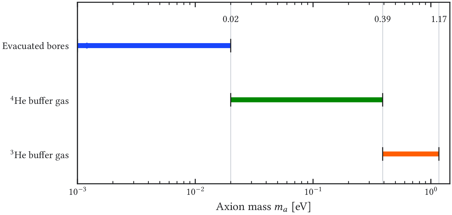
CAST separated the mass scan into three principal operating regimes, summarized in
Figure 2.6. The evacuated-bore phase retained coherence for \(m_a\lesssim 0.02\,\mathrm{eV}\). The first buffer-gas campaign used
\(\ce {^4He}\) at \(1.8\,\mathrm{K}\): 160 density settings, equivalent to pressure increments of approximately \(0.08\,\mathrm{mbar}\)
and reaching \(13.4\,\mathrm{mbar}\), covered \(0.02\text{--}0.39\,\mathrm{eV}\). The lower saturated-vapor pressure of \(\ce {^4He}\) limited the
accessible density. Replacing it with \(\ce {^3He}\) allowed higher pressures at the same
magnet temperature; successive scans covered \(0.39\text{--}1.17\,\mathrm{eV}\), with the pressure chosen so neighboring coherence
windows overlapped [49–51].
Figure 2.6: Axion-mass coverage of the principal CAST operating regimes. The vacuum
interval is set by loss of coherence in the \(9.26\,\mathrm{m}\) magnet. The \(\ce {^4He}\) and \(\ce
{^3He}\) intervals were scanned through many overlapping density settings; each
individual setting was resonant only over a narrow mass interval. End points summarize
the published campaign ranges and should not be interpreted as identical coupling
sensitivity throughout each interval [49–51].
CAST demonstrated low detector-background levels under helioscope conditions, the
background-count reduction obtained by focusing, and reliable long-term operation of a
Sun-tracking magnet and its detection lines. Its extended run with the IAXO pathfinder and a
xenon-based Micromegas detector found no axion signal and set \(\lvert g_{a\gamma }\rvert <5.8\times10^{-11}\,\mathrm{GeV}^{-1}\) at 95% confidence for \(m_a\lesssim 0.02\,\mathrm{eV}\) [40].
This result links the strongest demonstrated helioscope limit to the detector family,
focusing concept, and background-control methods developed further for the BabyIAXO
stage.
2.2.2 Why a Dedicated Helioscope Is Required
CAST also exposed the limitations of a repurposed accelerator magnet: small total aperture,
constrained detector and optics geometry, and limited tracking time. Because the figure of merit
depends on both the magnetic aperture and the detector–optics term, a substantial sensitivity
improvement requires a dedicated experimental design rather than incremental upgrades to an
existing accelerator component.
Parameter
CAST
BabyIAXO
IAXO
Magnet
concept
repurposed LHC
dipole
purpose-built
dipole
purpose-built
toroid
Representative
field
\(B\)
[T]
\(9\)
\(\sim 2\)
\(\sim 2.5\)
Magnetic
length
\(L\)
[m]
\(9.26\)
\(\sim 10\)
\(\sim 20\)
Total
aperture
\(A\)
[m2]
\(\sim 0.003\)
\(\sim 0.77\)
\(\sim 2.3\)
Magnet
FOM
\(f_M\)
[T2m4]
\(\sim 21\)
\(\sim 230\)
\(\sim 6000\)
Background
level
\(b\)
\(\sim 10^{-6}\)
\(\sim 10^{-7}\)
\(\sim 10^{-8}\)
Focal-region
area
\(a\)
[cm2]
\(0.15\)
\(2\times 0.3\)
\(8\times 0.15\)
Tracking
fraction
\(\epsilon _t\)
\(\sim 0.12\)
\(\sim 0.5\)
\(\sim 0.5\)
Table 2.1:
Published
conceptual-design
sensitivity
benchmarks
for
CAST,
BabyIAXO,
and
IAXO [12–14].
The
aperture
\(A\)
is
the
total
over
the
instrumented
bores,
and
the
entries
for
\(a\)
state
the
number
of
detection
lines
times
the
representative
area
per
line.
The
background
level
\(b\)
is
given
in
\(\unit {\counts \per \kilo \electronvolt \per \square \centi \meter \per \second }\).
The
quoted
\(f_M\)
values
come
from
detailed
magnetic-field
models
and
therefore
need
not
equal
the
result
obtained
from
the
rounded
values
of
\(B\),
\(L\),
and
\(A\)
shown
in
the
table.
The
CAST
detector
parameters
represent
the
IAXO-pathfinder
configuration
rather
than
every
detector
used
during
CAST.
Table 2.1 summarizes the resulting design shift. CAST exploited the high field of an accelerator
dipole, whereas BabyIAXO and IAXO exchange some field strength for much larger aperture,
systematic use of focusing optics, lower detector-background targets, and substantially longer solar
tracking. The IAXO strategy is therefore to co-optimize \(f_M\), \(f_{DO}\), and \(f_T\) in a purpose-built instrument [13,
46, 57].
2.3 The IAXO Experiment
2.3.1 Physics Reach and Design Philosophy
IAXO is conceived as a next-generation axion helioscope optimized for solar axions and ALPs [13,
45, 57]. In the low-mass region, design projections improve the background-limited signal-to-noise
ratio relative to CAST by approximately four to five orders of magnitude. They correspond to a
projected sensitivity near \(\lvert g_{a\gamma }\rvert \sim 3\times10^{-12}\,\mathrm{GeV}^{-1}\), approximately a factor of 20 below the current CAST limit, subject
to the assumed exposure and background performance [45]. The observatory is also
designed to probe solar production through \(g_{ae}\) with sensitivity beyond previous laboratory
searches.
Figure 2.7: Helioscope-relevant axion–photon parameter space. The CAST and
stellar-cooling bounds and the BabyIAXO/IAXO projection curves are redrawn from
checksum-verified data in the AxionLimits snapshot pinned to Git commit
7d375f4 [39]. The original CAST and globular-cluster results are given in Refs. [40, 41],
and the conceptual-design projections in Refs. [14, 58]. Solid boundaries with shading
denote observed exclusions, whereas unfilled dashed or dotted curves denote
heterogeneous design projections. The hatched QCD-axion band uses the central
mass–coupling constants in Eqs. 1.4 and 1.5 and is not an exclusion [8]. Within it, the
solid and dashed brown lines mark the KSVZ (\(E/N=0\)) and DFSZ (\(E/N=8/3\)) benchmark relations,
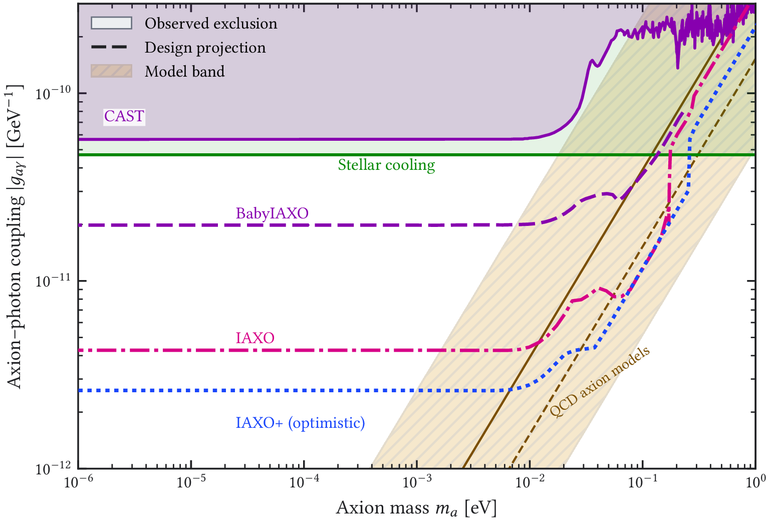
respectively. IAXO+ denotes the optimistic ultimate reach of the IAXO
research-and-development program, not a separately approved experimental stage [58].
These projections set the performance targets for the coupled subsystems discussed
below: magnetic conversion aperture, X-ray optics and focal-plane background, and
solar-tracking exposure. The IAXO+ curve is retained only as an optimistic performance
benchmark; the baseline experimental stages discussed in this thesis are BabyIAXO and
IAXO. The projection curves reproduce heterogeneous literature assumptions and were
not recalculated from the March 2026 engineering parameters. Observed boundaries
are digitized approximations; the current published CAST plateau is the \(5.8\times10^{-11}\,\mathrm{GeV}^{-1}\) limit quoted
above.
2.3.2 Magnet
The 2014 reference design for IAXO uses a superconducting toroidal magnet approximately \(20\,\mathrm{m}\) long,
formed by eight coils and providing eight bores of approximately \(60\,\mathrm{cm}\) diameter [13]. The useful field
in the bores is approximately \(2.5\,\mathrm{T}\), while the peak field in the windings is about \(5.4\,\mathrm{T}\); the principal gain
over CAST comes from the much larger integrated magnetic aperture. The toroidal
layout leaves the bores accessible for optics and detectors and defines eight parallel
detection lines. The bores can operate in vacuum or, for higher-mass scans, with a buffer
gas.
The final magnet design remains part of the post-BabyIAXO program. Recent studies retain the
large multi-bore concept while also considering high-temperature-superconductor alternatives that
could change the field and cryogenic implementation [45].
2.3.3 X-ray Optics
The reference IAXO design equips every detection line with grazing-incidence X-ray optics [13,
59]. The sensitivity benchmark in Table 2.1 assumes a selected focal-region area of approximately \(0.15\,\mathrm{cm}^{2}\)
per line. Detailed designs optimize both the energy-dependent throughput and the focal image of
the extended solar source.
Focusing does not reduce the areal detector background level \(b\). Instead, it confines the
signal to a small selected area \(a\), reducing the expected background counts in the signal
region in proportion to \(ba\) when the background is approximately uniform. This coupling
between optics and detector performance is the origin of the detector–optics term in
Equation 2.6.
2.3.4 Detector Technologies
The focal-plane detectors must combine high efficiency in the reference \(1\text{--}10\,\mathrm{keV}\) band with
stage-dependent background targets. The BabyIAXO sensitivity benchmark assumes a background
level of \(1\times10^{-7}\,\mathrm{counts}\,\mathrm{keV}^{-1}\,\mathrm{cm}^{-2}\,\mathrm{s}^{-1}\), whereas the full IAXO concept targets \(1\times10^{-8}\,\mathrm{counts}\,\mathrm{keV}^{-1}\,\mathrm{cm}^{-2}\,\mathrm{s}^{-1}\) [13, 14]. Under the surface conditions considered
for the program, meeting these targets requires radiopure construction, passive shielding,
topology-based discrimination, and active-veto systems [17].
Microbulk Micromegas detectors are the most developed gaseous technology for this role
because CAST and IAXO-D0 demonstrated their radiopurity, topological discrimination, stable
operation, and compatibility with focused soft X rays. Alternative focal-plane concepts include
GridPix detectors, metallic magnetic calorimeters, transition-edge sensors, and silicon drift
detectors; their lower thresholds or improved energy resolution are particularly relevant to the
softer ABC spectrum [45, 60, 61]. Chapter 3 develops the Micromegas detector line used in this
thesis.
2.3.5 Tracking and Observatory Operation
The reference IAXO concept mounts the magnet, optics, and detectors on elevation and azimuth
drives that provide solar tracking for up to approximately half of each day, corresponding to \(\epsilon _t\simeq 0.5\) [13].
The moving structure must support the cold mass, preserve alignment among the bores, optics, and
detectors, and allow reproducible transitions between Sun-tracking data and off-Sun background
measurements. These requirements enter both the sensitivity exposure and the background-control
strategy.
The conceptual installations are surface facilities rather than deep-underground
laboratories. Background suppression must therefore be obtained through the detector,
passive shielding, event-topology analysis, and active vetoing. The evolution of the
specific BabyIAXO site assumption, and its consequences for this thesis, are discussed
below.
2.4 BabyIAXO as an Intermediate Stage
2.4.1 Role Within the IAXO Program
BabyIAXO is the intermediate experimental stage between CAST and the full IAXO
observatory [14, 45, 58]. It provides a common environment in which the magnet, optics,
detectors, cryogenics, tracking, alignment, gas handling, and data acquisition can be integrated and
commissioned. At the same time, it is a physics instrument with independent discovery reach. This
staged program also builds the shared analysis, software, operations, and system-integration
experience required for the full observatory.
Under the 2021 conceptual-design assumptions, including \(1.5\,\mathrm{yr}\) of effective exposure for each of the
vacuum and buffer-gas campaigns, the projected low-mass vacuum sensitivity is \(\lvert g_{a\gamma }\rvert \simeq 1.5\times10^{-11}\,\mathrm{GeV}^{-1}\) for \(m_a\lesssim 0.02\,\mathrm{eV}\).
The projected buffer-gas scan would extend the reach to higher masses and probe the
KSVZ benchmark approximately over \(0.06\text{--}0.25\,\mathrm{eV}\) [14]. BabyIAXO therefore combines new physics
reach with validation of the technologies and subsystem interfaces required for the full
observatory.
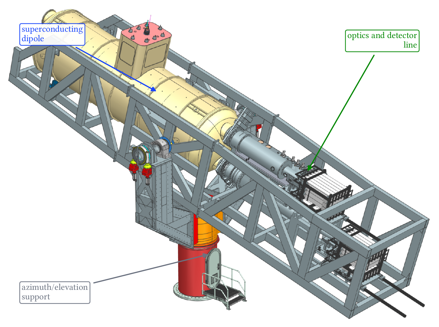
Figure 2.8: Annotated view of the current BabyIAXO integration model, adapted from the
March 2026 superconducting-dipole status presentation [62]. The rendering identifies the
superconducting dipole, one optics–detector line, and the azimuth–elevation support used
for solar tracking.
2.4.2 Main Experimental Features
The 2021 conceptual design established a common-coil dipole with two parallel flat racetrack coils
carrying opposite currents and two \(10\,\mathrm{m}\)-class bores [14]. By March 2026, the engineering
model specified two \(11\,\mathrm{m}\)-long free bores of \(0.70\,\mathrm{m}\) diameter and an aluminum-stabilized NbTi/Cu
Rutherford-cable conductor operated at \(6\,\mathrm{kA}\) [62]. At that operating current, the calculated mean
transverse bore field is \(2.1\,\mathrm{T}\), the peak field on the cable is \(4.7\,\mathrm{T}\), and the three-dimensional magnet
figure of merit is approximately \(290\,\mathrm{T}^{2}\,\mathrm{m}^{4}\). The public June 2026 status presentation retained these
engineering values [63]. Each bore can host a complete detection line with dimensions
representative of the full observatory, allowing the magnet aperture, cryogenic integration, and
detector interfaces to be tested at full line scale before the final toroidal observatory is
designed.
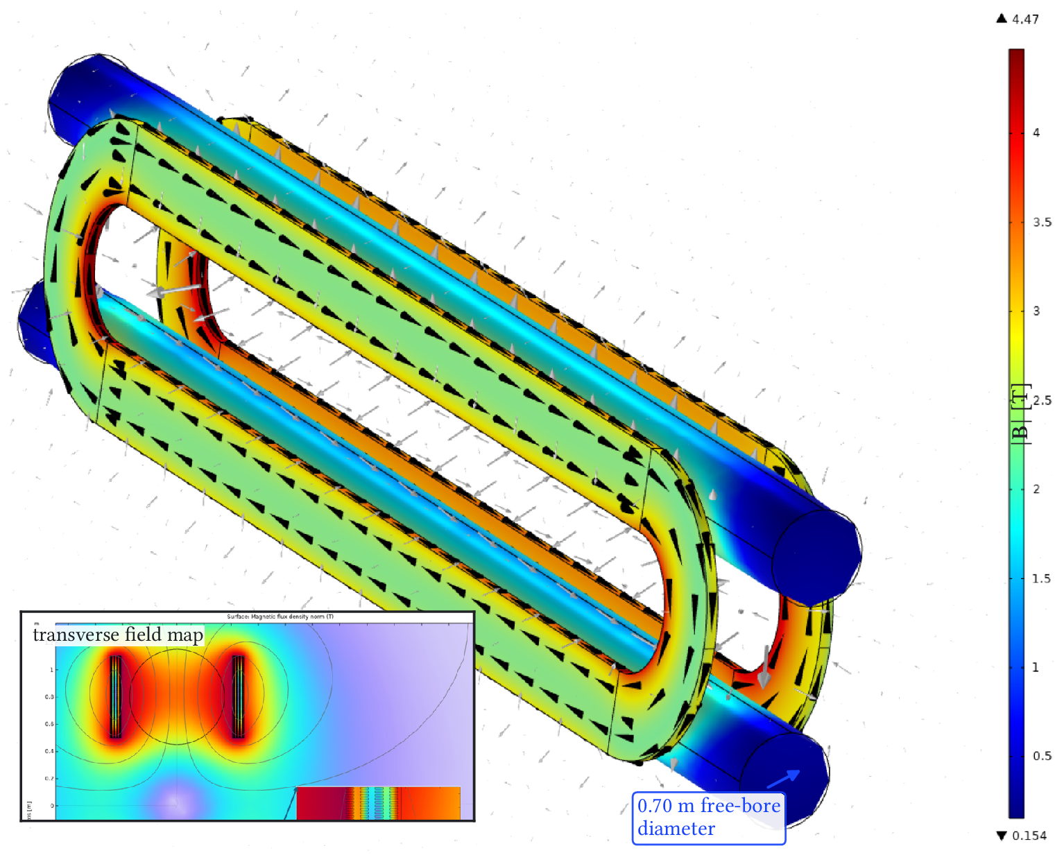
Figure 2.9: Three-dimensional magnetic-field model of the current BabyIAXO common-coil
dipole, adapted from the March 2026 superconducting-dipole status presentation [62].
Color encodes the field magnitude \(\lvert \mathbf {B}\rvert \) in tesla, and the inset provides a transverse field-map
detail through the straight coil sections. The peak field occurs in the conductor and must
not be confused with the \(2.1\,\mathrm{T}\) mean transverse field in the two \(0.70\,\mathrm{m}\)-diameter free bores.
On August 11, 2026, the University of Bonn announced approval of a magnet system costing
EUR 6 million, financed by EUR 3 million from the German Research Foundation (DFG),
EUR 2.4 million from North Rhine-Westphalia, and EUR 0.6 million from the participating
universities [64]. This funding milestone concerns magnet construction; it does not establish
completion of the magnet or approval of the final DESY site.
The 2021 conceptual optics baseline paired one custom, NuSTAR-derived segmented-glass
telescope with an available XMM-Newton flight-spare telescope [14]. By the 23rd IAXO
Collaboration Meeting in March 2026, the optics program also included BRAVO-SUN and
XRISM-derived components and was developing a co-mounted telescope configuration. The
final combination of components remained under development [65]. The June 2026
public comparison quoted approximately \(0.2\,\mathrm{cm}^{2}\) for the custom telescope and \(0.3\text{--}0.7\,\mathrm{cm}^{2}\) for the XMM
telescope [63]. These areas cannot be applied interchangeably: each line requires its own
energy-dependent throughput and focal containment, evaluated for the chosen signal
region.
Micromegas remain the principal low-background technology for the detector line studied
here, while the broader BabyIAXO program also develops GridPix and cryogenic focal-plane
detectors [14, 61]. The detector line treated in this thesis is therefore one implementation within a
broader focal-plane program.
2.4.3 Evolution of the DESY Site Scenario
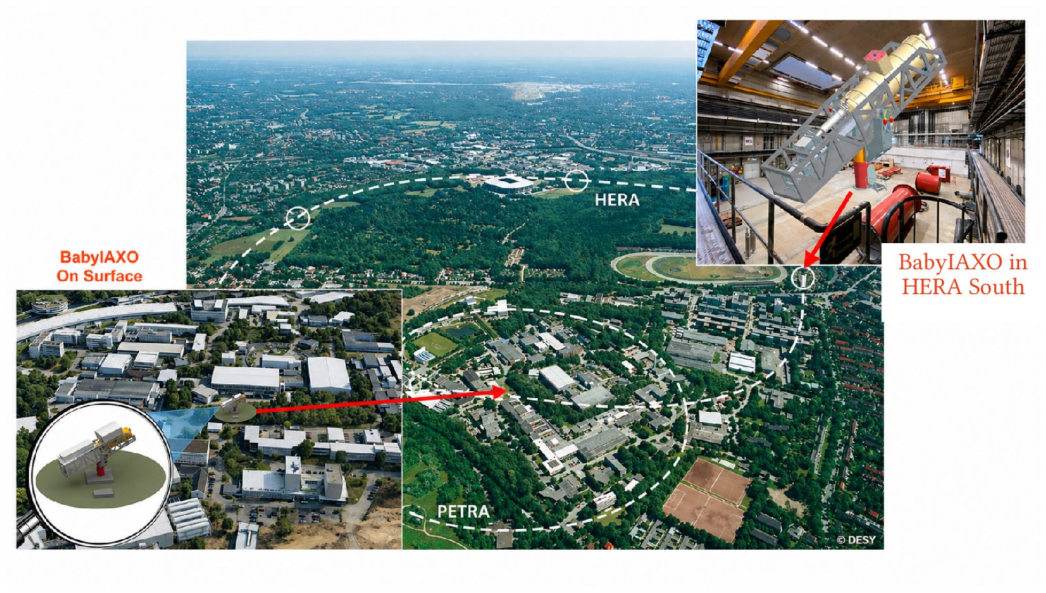
When the background-model and veto-simulation program began, the reference BabyIAXO site
was the HERA South Hall on the DESY campus. The hall is an underground accelerator space
rather than a deep-underground low-background laboratory, but its structure, access shafts, and
surrounding material could modify the cosmic-ray field relative to an outdoor installation. Early
simulations therefore treated the cosmic-ray component as site dependent, with attention to
overburden, openings, and local shielding.
During 2025 and 2026, internal collaboration studies shifted the working baseline
toward an outdoor, on-surface location on the DESY campus. The reported considerations
included simpler civil infrastructure, reduced demands on DESY infrastructure resources,
lower expected cost, and a shorter route to site activation [67]. As reported at the 23rd
collaboration meeting in March 2026, the DESY directorate had encouraged further
site exploration and development of cost and schedule plans. This did not constitute
formal project or site approval, and the exact position and site elevation remained under
study [15].
The March 2026 on-surface working baseline is adopted here without credit for hall
overburden. Simulations that retain boundary conditions associated with HERA South are
identified separately. An outdoor source spectrum is not a demonstrated upper bound on every
local contribution: the ground, housing, platform, and magnet can attenuate primaries while
generating or redistributing secondaries. Transfer to the final site therefore requires a consistently
normalized source boundary and transport through the local environment. The detector system
must address sea-level muons, neutrons, and secondary particle production in the passive
shielding. An active veto is therefore central to the mitigation strategy investigated here;
Chapter 5 evaluates the proposed plastic-scintillator veto with cadmium neutron-capture
layers.
2.5 Connection to the Present Thesis
Chapter 3 narrows the discussion from the helioscope to the detector-development line. It
introduces time-projection-chamber signal formation and microbulk Micromegas technology, then
describes the IAXO-D0 experimental prototype and the IAXO-D1 simulation geometry used in this
work. Chapter 4 develops the REST-for-Physics/restG4 framework used to represent
that detector and its environment. Chapters 5 and 6 evaluate the active-veto strategy and
assemble the validated components and remaining limitations of the partial background
model.
Chapter 3 Micromegas X-ray Detectors for BabyIAXO
Introduction
The Micromegas detector line studied in this thesis is the low-background X-ray detection system
coupled to the BabyIAXO helioscope optics. Its task is narrow but demanding: it must convert a
small number of soft X rays in the \(1\)–\(10\,\mathrm {keV}\) region into calibrated, position-sensitive waveforms while
operating at surface level, close to passive shielding, active veto panels, gas services,
high-voltage channels, and data-acquisition electronics. For that reason, the detector
cannot be described only as an isolated gas volume. It is a coupled instrument in which
gas transport, charge amplification, readout segmentation, calibration, slow control,
and veto synchronization all determine the observables used later in the background
analysis.
This chapter provides the detector foundation for the rest of the thesis. It first summarizes the
signal-formation physics that is needed to interpret Micromegas waveforms, then describes the
microbulk Micromegas technology and the IAXO-D0/IAXO-D1 prototype implementations. The
final sections connect the detector to its operating services, data-acquisition chain, and calibration
procedures, leaving the detailed software implementations and large-scale background simulations
to Chapters 4 and 6.
3.1 The Time Projection Chamber (TPC)
Time Projection Chambers (TPCs) are gaseous detectors in which ionization electrons drift
through an electric field toward a segmented readout plane. Large TPCs are often used as tracking
detectors, but the BabyIAXO Micromegas detector is a shallow X-ray TPC: the relevant
information is not a long momentum-measuring trajectory, but the amount of deposited charge,
its two-dimensional distribution on the readout strips, and the relative timing of the
digitized pulses. This compact topology is precisely what makes the detector useful for
axion searches, because focused solar X rays should produce localized charge clusters
while many background events produce more extended, asymmetric, or veto-correlated
signatures.
A TPC typically consists of a gas-filled chamber subjected to a uniform drift field. An incoming
particle or photon interaction produces electron-ion pairs in the gas. The electrons drift toward
the anode, diffuse during transport, enter an amplification region, and finally induce
signals on the readout electrodes. The ions drift more slowly toward the cathode. In the
BabyIAXO detector, the readout plane is a microbulk Micromegas, which combines
amplification and fine strip segmentation in a radiopure structure suitable for low-background
operation.
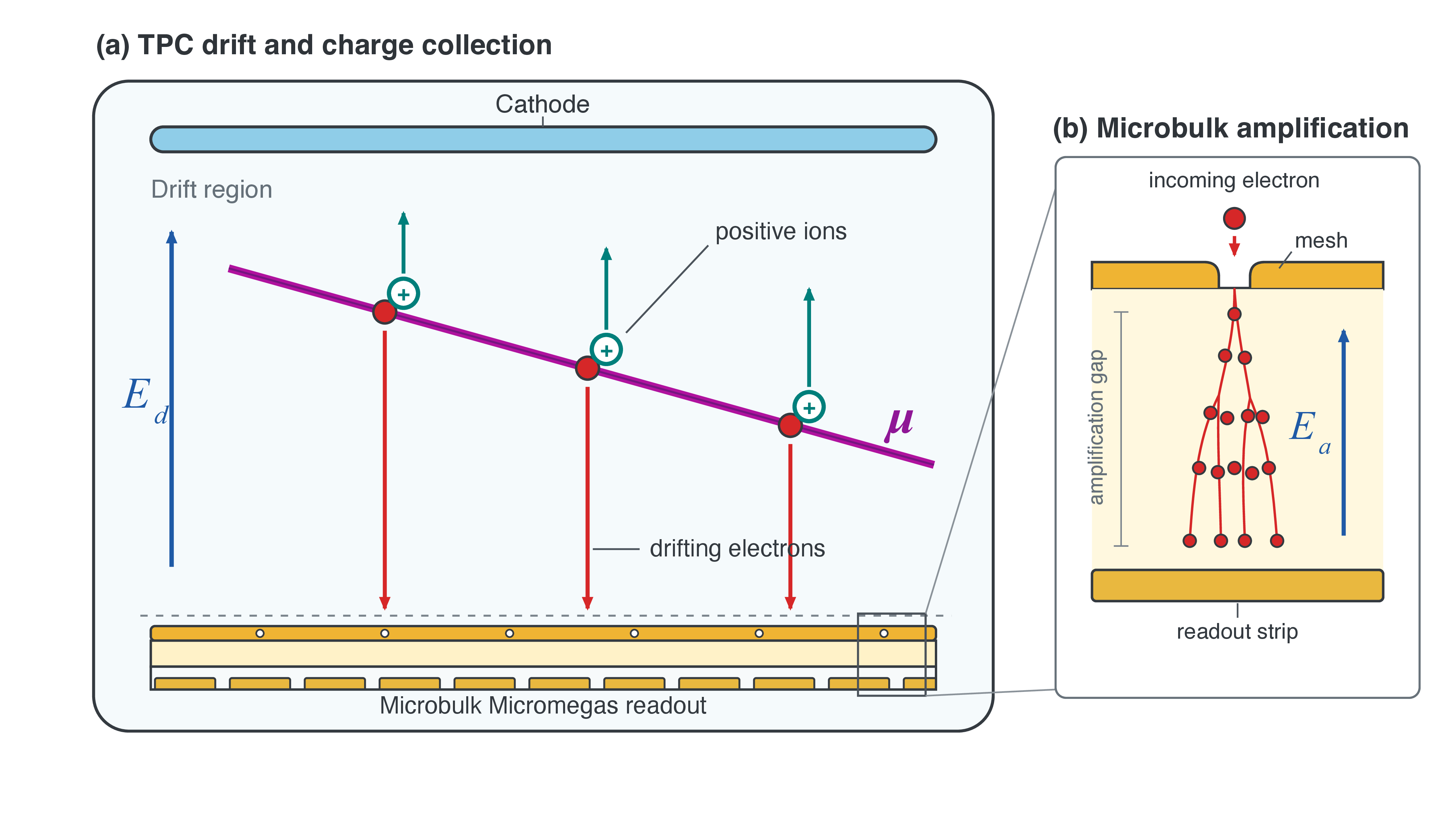
Figure 3.1: Schematic representation of a Time Projection Chamber (TPC). The ionization
of the gas medium by an incoming particle results in the generation of electrons. The
electrons drift toward the anode under the influence of an electric field \(E_d\) and are amplified
upon reaching the amplification region where a higher electric field \(E_a\) is applied.
3.1.1 Ionization in Gases
The Micromegas signal starts with an energy deposition in the gas. For the soft X rays relevant to
BabyIAXO this deposition is dominated by photoelectric absorption, whereas charged particles
usually produce extended ionization tracks and neutral particles contribute indirectly through
recoils or secondary radiation. Only the aspects of these processes that determine the later
waveform and calibration response are summarized here.
For photons, the attenuation through a material is described by
Here, \(\mu \) is the linear attenuation coefficient. Equivalently, \(\mu =\rho \mu _m\), with \(\mu _m\) the mass attenuation coefficient.
In the few-keV signal region, the photoelectric effect dominates the attenuation and produces a
localized primary-electron cloud. The full background simulation transports the other
electromagnetic processes, but they are not needed to explain the calibration and signal topology
developed in this chapter.
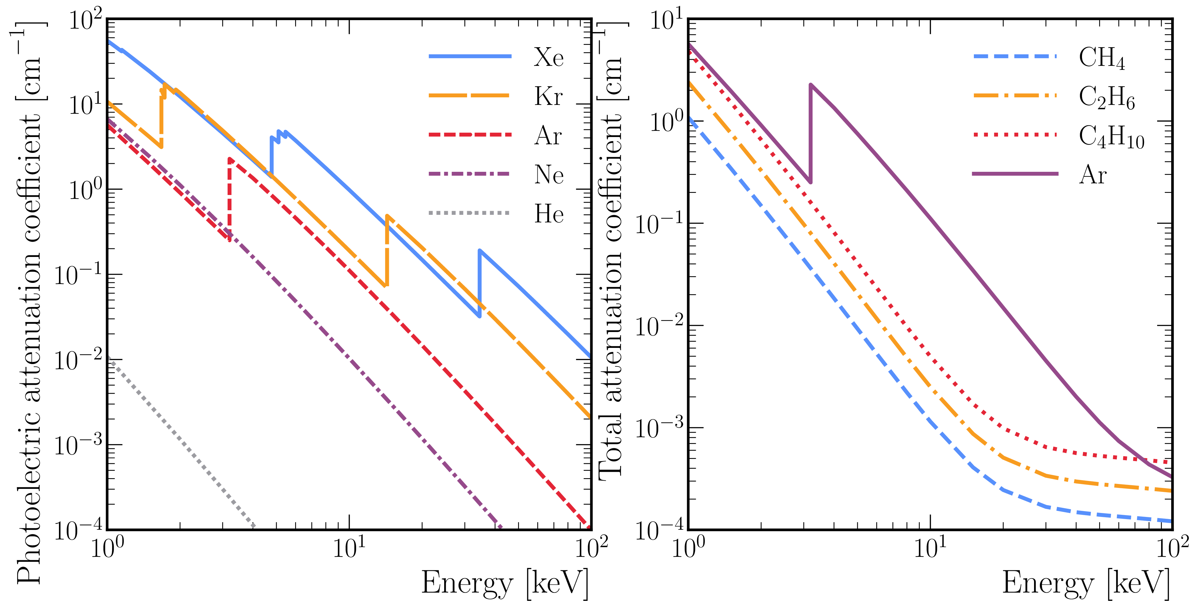
Figure 3.2: Photoelectric attenuation coefficient for noble gases as a function of energy
(left) and total attenuation coefficient for some saturated hydrocarbons, commonly used in
gaseous mixtures as quenchers, with argon for comparison (right). Data from [68]
evaluated at a temperature of \(25~^{\circ }\mathrm {C}\) and a pressure of \(1~\mathrm {bar}\).
The preference for noble gases follows directly from the strong \(Z\) dependence of the
photoelectric cross section in the X-ray range, visible in Figure 3.2. The quencher is
present at much lower concentration and has a smaller attenuation contribution, but it is
essential for stable proportional operation. After photoelectric absorption, the atomic
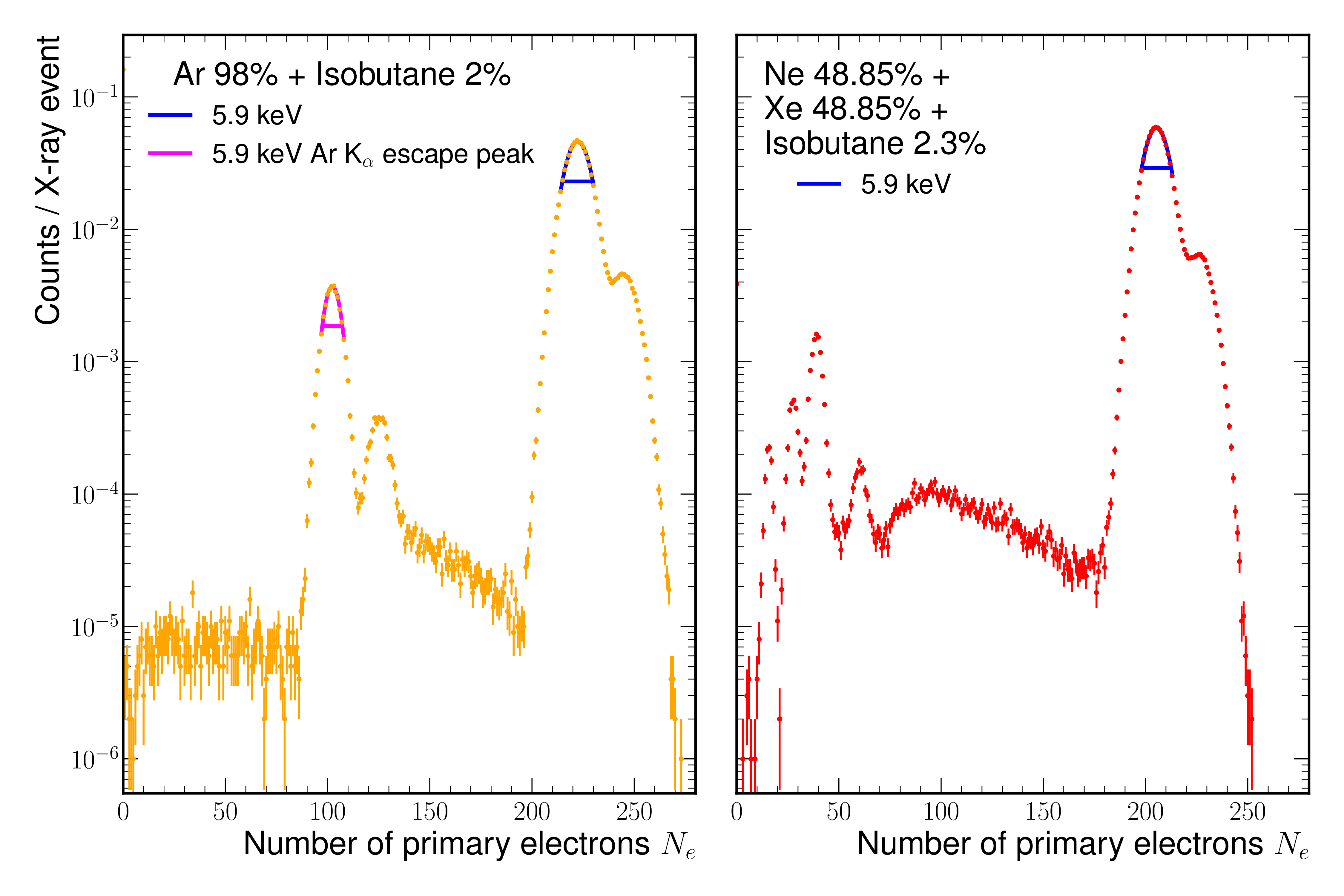
vacancy relaxes through Auger emission or fluorescence. If a fluorescent x ray escapes the
sensitive volume, the measured energy is reduced and an escape feature appears in the
calibration spectrum; this is particularly visible for argon-based \(\ce {^{55}Fe}\)
calibrations.
Charged particles instead leave ionization along their path, with a topology governed by the
stopping power, multiple scattering, and possible secondary radiation. In a Micromegas TPC this
typically produces broader and more track-like charge patterns than a few-keV X ray. Neutral
particles are relevant because they can generate nuclear recoils or secondary photons and charged
particles in the gas or surrounding materials. This indirect character is one of the reasons why the
background model treats radiation transport and detector-response reconstruction together rather
than as separable problems.
3.1.2 Electron Transport
Primary Charge Production
An electron-recoil energy deposit \(E\) in the gas produces a finite number of electron-ion pairs. The
electrons, referred to here as primary charge, are the carriers that drift toward the Micromegas
readout and seed the avalanche in the amplification gap. The mean number of primary electrons
is
Here, \(W\) is the average energy required to create one electron-ion pair in the mixture. For nuclear
recoils, part of the kinetic energy goes into atomic motion rather than ionization, so the
corresponding charge yield requires a recoil-response model, discussed in Appendix C.1.2. The
intrinsic fluctuation around this mean is smaller than Poissonian and is commonly written
as
\begin{equation} \sigma _e^2 = F N_e. \label {fano_variance} \end{equation}
Here, \(F\) is the Fano factor [69]. This primary-charge statistics sets the best achievable energy
resolution before transport, amplification, and electronics effects are included.
Electron Drift
The drift field transports the primary electrons from the conversion point to the amplification
region. In the mobility approximation, the drift velocity can be written as
Here, \(\mu _e>0\) is the magnitude of the electron mobility at the operating field, gas density, and
composition; the minus sign expresses motion opposite to \(\vec {E}\). At fixed temperature, transport tables
are conveniently compared using the reduced field \(E/p\), where \(p\) is the pressure; \(E/N\), with \(N\) the gas
number density, is the more general variable when temperature changes. In practice, drift
velocities and diffusion coefficients are taken from gas-transport calculations such as
Garfield++/Magboltz, because the response depends on the mixture, pressure, field, and
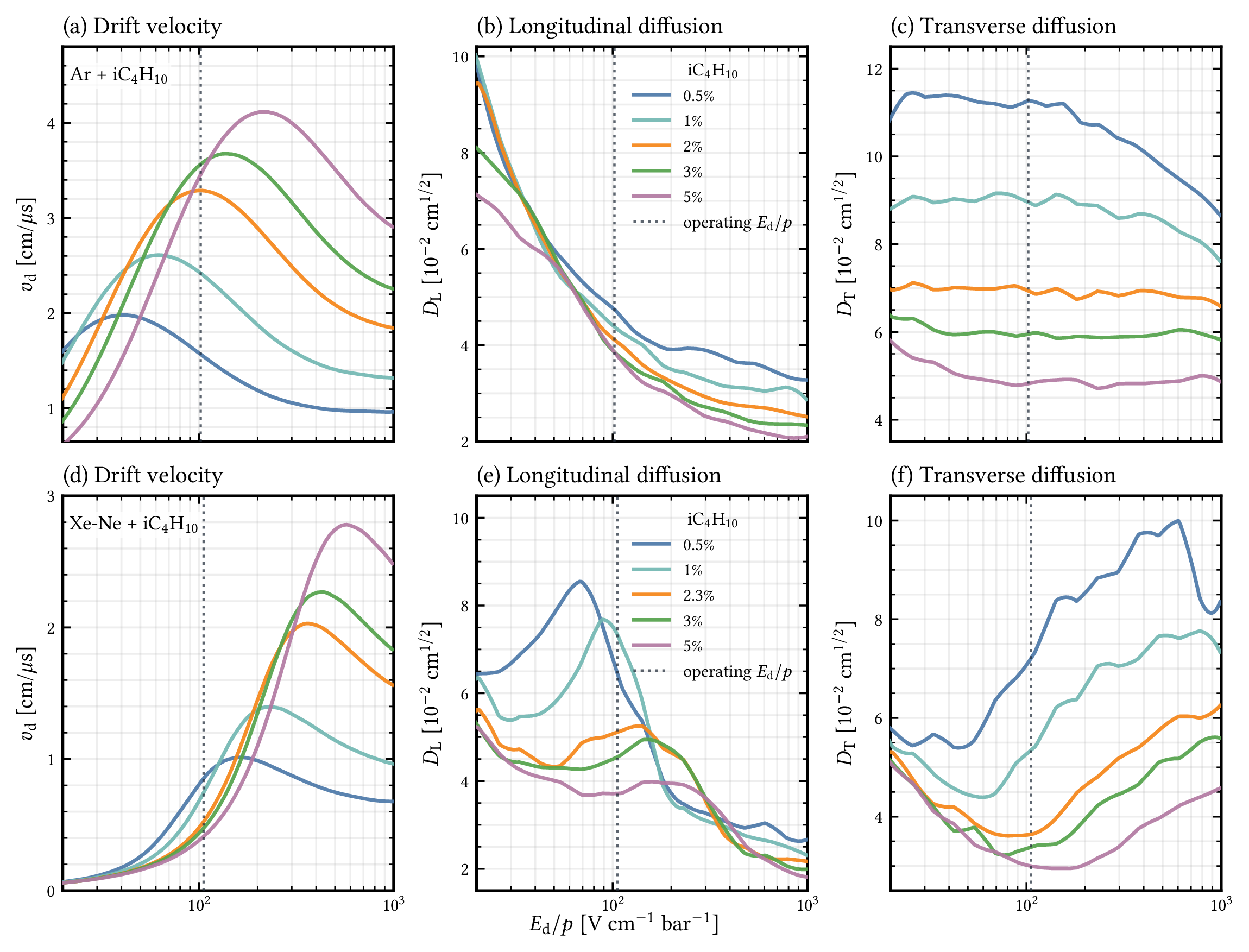
quencher fraction. Typical electron drift velocities in noble-gas TPC mixtures are of order \(1\,\mathrm{cm}\,\mathrm{\mu s}^{-1}\), so the
drift time is directly connected to the pulse timing in the digitized waveform. The gas-mixture
dependence of the drift velocity and diffusion coefficients is discussed below in the context of the
detector-response gas tables.
During transport the charge cloud also diffuses. The standard deviation \(\sigma _{\hat {u}}\) of the electron cloud in
a given direction \(\hat {u}\) after a drift distance \(d\) can be written as
The coefficients \(D_{\hat {u}}\) in this convention have units of square-root length, as in the Garfield++
gas tables [70]. They are related to the conventional diffusion coefficients \(\mathcal {D}_{\hat {u}}\), with units of length
squared per time, by \(D_{\hat {u}}=\sqrt {2\mathcal {D}_{\hat {u}}/|\vec {v}_d|}\) for uniform drift.
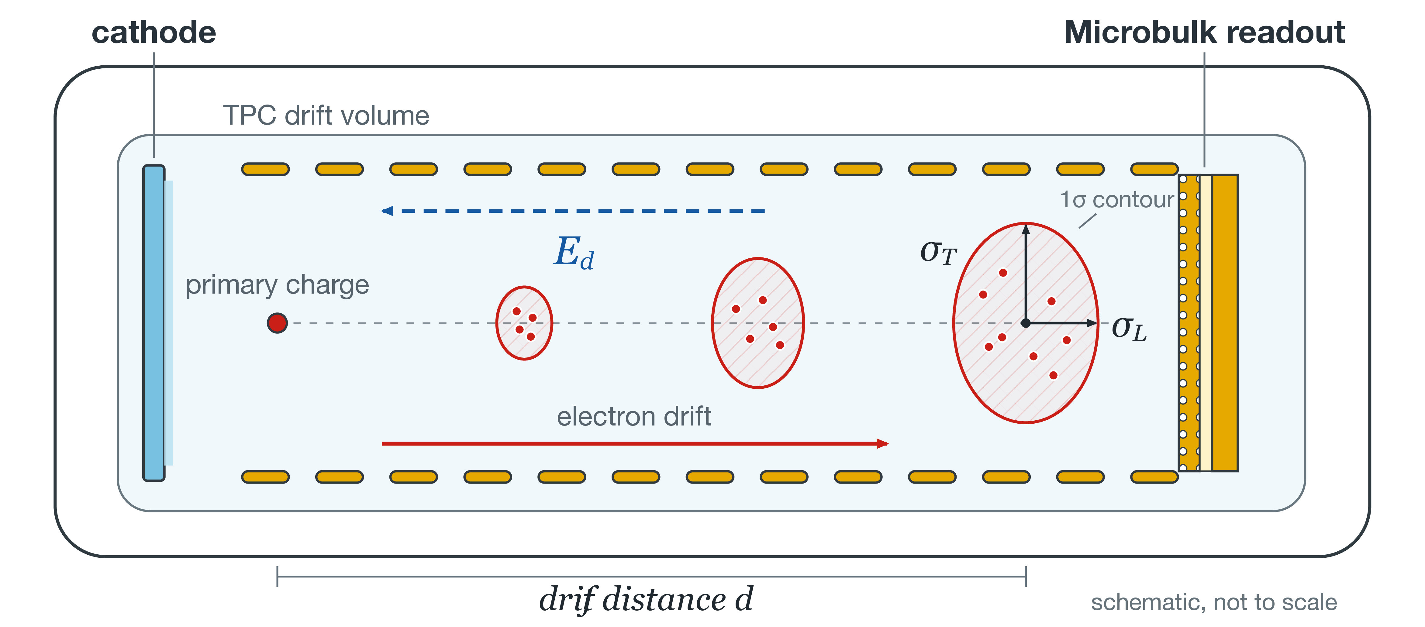
Figure 3.3: Technical cutaway of electron diffusion in a TPC. Successive outlined and
hatched contours show the growth of the one-standard-deviation envelope as primary
charge drifts toward the Microbulk readout. In the final cloud, \(\sigma _L\) is measured parallel to the
mean drift direction and \(\sigma _T\) perpendicular to it; both arrows extend from the centroid to the
one-standard-deviation contour and therefore denote semi-axes.
In the longitudinal section shown in Figure 3.3, the primary charge drifts opposite to the
electric field. The longitudinal width \(\sigma _L\) is parallel to the mean drift direction, whereas the transverse
width \(\sigma _T\) is perpendicular to it. Both are defined from the charge-cloud centroid to its
one-standard-deviation contour; they are therefore semi-axes of the contour, not full cloud
diameters. The separate longitudinal and transverse diffusion coefficients arise in the presence of
the drift field. Diffusion controls the charge sharing between strips and the apparent width of a
localized X-ray event. Recombination and attachment provide the competing loss mechanisms; in
practice, oxygen and water contamination are the main operational concerns, which is why gas
purity, material outgassing, and circulation are part of the detector response rather than purely
auxiliary services.
Charge Amplification
The primary charge is too small to be measured directly, so the Micromegas gap operates in
avalanche mode. The high amplification field converts each primary electron into a charge packet
whose mean size is set by the gas gain.
The mean electron population \(N_a\) after amplification of \(N_e\) primary electrons across a gap of length \(L\)
is, when attachment is negligible,
Here, \(\alpha \) is the first Townsend coefficient, which depends on the gas medium and the electric field.
The number of electrons after amplification of the primary charge \(N_a\) can be expressed
as
\begin{equation} N_a = G N_e. \label {gain-definition} \end{equation}
If the gain fluctuations of individual primary electrons are described by a variance \(\sigma _G^2\), the
variance of the amplified electron population, \(\sigma _a^2\), can be written as
\begin{equation} b = \frac {\sigma _G^2}{G^2}. \end{equation}
For an approximately Gaussian peak, the resolution \(R = 2 \sqrt {2 \ln {2}} \sigma _a / N_a \approx 2.35 \cdot \sigma _a / N_a\) is the full width at half maximum (FWHM)
of the amplified-charge distribution divided by its mean value.
\begin{equation} R \approx 2.35 \sqrt { \frac {1}{N_e} \left ( F + b \right ) + \left (\frac {\sigma _{\mathrm {el}}}{G N_e}\right )^2 } \label {resolution_fwhm} . \end{equation}
Here, \(\sigma _{\mathrm {el}}\) represents additional electronic-noise contributions referred to the amplified
charge. The expression assumes independent single-electron avalanches and additive noise
uncorrelated with the primary charge [71]. The resolution \(R\) is commonly expressed as a
percentage.
Figure 3.4: Simplified primary-charge simulation for X rays from a \(\ce
{^{55}Fe}\) source in a \(6\,\mathrm{cm}\times6\,\mathrm{cm}\times3\,\mathrm{cm}\) gas volume. The photons are emitted from the center of one \(6\,\mathrm{cm}\times6\,\mathrm{cm}\)
face toward the geometric center of the volume. For the argon mixture the pressure is \(1.4\,\mathrm{bar}\) and
the drift field is \(135\,\mathrm{V}\,\mathrm{cm}^{-1}\); for the xenon mixture they are \(1.05\,\mathrm{bar}\) and \(110\,\mathrm{V}\,\mathrm{cm}^{-1}\), respectively. Both mixtures are
evaluated at \(20\,\mathrm{{}^{\circ}C}\). Gaussian fits to the main primary-charge peaks give centroids of 222.29 and
205.35 electrons and absolute FWHM values of 15.05 and 14.43 electrons for argon and
xenon–neon, respectively. The corresponding relative resolutions are \(R=6.77\%\) and \(7.03\%\), obtained by
dividing each width by its centroid. Error bars show 68.27% Garwood intervals on the
simulated bin counts, divided by the total sample size. The argon escape structure is visible
at lower charge; the zero-electron population includes photons that do not produce
collected primary ionization in this simplified volume.
Expression 3.10 separates the primary-ionization and avalanche contributions from electronic
noise, which becomes increasingly important near threshold. The approximately \(7\%\) primary-only
FWHM in Figure 3.4 is an intrinsic reference for these gas mixtures and this X-ray energy. It
excludes amplification, charge loss and readout fluctuations and therefore is not the predicted
resolution of the complete detector. Measured microbulk resolutions also depend on gain and
collection conditions [72].
Avalanche ultraviolet photons can initiate secondary avalanches by photoionizing gas species
or releasing electrons from surfaces. Adding isobutane suppresses this feedback through
absorption and non-radiative molecular relaxation. The quencher also changes charge transport, as
illustrated in Figure 3.5.
Figure 3.5: Effect of the isobutane quencher fraction on Micromegas gas-transport
properties, computed with Garfield++/Magboltz gas tables at \(20\,^{\circ }\mathrm {C}\) [70]. The upper row
shows argon–isobutane mixtures and the lower row shows equal-partial-pressure
xenon–neon mixtures with isobutane. The curves are plotted as a function of the reduced
drift field in bar units, \(E_d/p\). The vertical dotted line in each row marks the representative
operating point used to read the transport properties in the detector-response studies: the
center of the \(E_d \simeq 133\)–\(153\,\mathrm {V/cm}\) range at \(p=1.4\,\mathrm {bar}\) for the argon mixtures, and \(E_d \simeq 111\,\mathrm {V/cm}\) at \(p=1.05\,\mathrm {bar}\) for the xenon–neon mixture. The \(2\%\)
argon–isobutane curve is a representative detector-response scan rather than the frozen
background-model gas: the conservative IAXO-D1 reference in Chapter 6 uses
argon–isobutane at \(1\%\), while the \(2.3\%\) xenon–neon–isobutane mixture belongs to the separate
BabyIAXO response studies.
Increasing the isobutane fraction generally reduces transverse diffusion in these scans,
producing a narrower cloud after the same drift distance. Changes in drift velocity and longitudinal
diffusion also affect the relation between waveform timing, drift position, and the extent of a
localized ionization cluster. The dotted lines mark reference operating fields, rather than
gas-optimization boundaries. Gas choice must therefore balance charge transport, attachment,
amplification stability, and operational requirements. The calculation workflow is described in
Section 4.6.6.
3.1.3 Micropattern Gaseous Detectors: Micromegas
Micromegas (MICRO-MEsh GAseous Structure) detectors are micropattern gaseous detectors in
which a thin metallic mesh separates the drift region from a narrow amplification gap [73].
Ionization electrons produced in the drift volume pass through the mesh when the field ratio
between amplification and drift regions is favorable, and then avalanche in the high-field gap
before being collected by the anode strips. This separation between a relatively low-field
drift volume and a very high-field amplification region gives Micromegas detectors fast
signals, good spatial granularity, and stable operation at gains suitable for soft X-ray
detection.
For axion helioscopes and other rare-event searches, the relevant implementation is the
microbulk Micromegas. In this technology the mesh, insulating pillars, and readout pattern are
manufactured from copper-clad kapton using photolithographic processes, producing a thin and
mechanically uniform amplification structure [74]. The small material budget, the use of radiopure
copper and kapton, and the possibility of producing fine two-dimensional strip readouts are central
advantages for low-background X-ray detectors. They also make the detector naturally compatible
with a TPC analysis strategy: X-ray events produce compact clusters, while tracks from
cosmic rays or radioactive backgrounds tend to be more extended in at least one strip
projection.
Three distinct length scales should not be conflated. The \(6\,\mathrm{cm}\)-wide IAXO readout contains 120
strips per coordinate, giving a strip pitch of \(500\,\mathrm{\mu m}\). At each X–Y strip crossing, the IAXO-D1 mesh
photograph shows a \(3\times 3\) group of microscopic openings. Microbulk structures of this detector family
use holes of order \(40\,\mathrm{\mu m}\) in diameter on an approximately \(100\,\mathrm{\mu m}\) triangular pitch, while the etched polyimide
defines an amplification gap of approximately \(50\,\mathrm{\mu m}\) [56, 72]. The strip pitch sets the two-dimensional
readout granularity; the much smaller hole pitch and gap determine electron transmission and
avalanche formation.
The operating point of a Micromegas detector is defined by the drift field, mesh voltage, gas
mixture, pressure, and readout threshold. The mesh transparency must be high enough that
primary electrons enter the amplification gap efficiently, while the gain must be large
enough to resolve keV deposits without approaching unstable discharge conditions. These
two requirements are coupled: the field ratio controls electron focusing through the
mesh, while the amplification field controls both signal size and discharge probability.
Consequently, stable operation is not only a matter of setting a high voltage, but of choosing a
consistent gas, voltage, and electronics configuration and monitoring it through calibration
data.
The combination of radiopurity, segmentation, low threshold, and successful operation in
CAST makes microbulk Micromegas the baseline detector technology for the IAXO Micromegas
line [12, 16, 40].
Figure 3.6: Simplified design of a microbulk Micromegas readout, showing the orthogonal
X and Y strip pixels and a cut-out of the perforated copper mesh above them. The design is
based on the BabyIAXO readout in Figure 3.10, but it contains \(8+8\) strips instead of \(120+120\). The
X-strip pixels are connected in the same PCB layer, while the Y-strip pixels are connected
through the bottom layer. In the real detector, the mesh is separated from the readout by an
approximately \(50\,\mathrm{\mu m}\) amplification gap; the full TPC drift region lies above the mesh and is not
shown.
3.2 The BabyIAXO Micromegas Detector Prototypes
The baseline detector technology for IAXO and BabyIAXO is the microbulk Micromegas. Its
successful operation in CAST, where it provided low-background X-ray detection for the
solar-axion search, makes it the established baseline choice for the IAXO program.
The TPC design of the BabyIAXO Micromegas detector remains similar to the CAST
Micromegas detectors, since both experiments are designed with the same goal of detecting solar
axions. The gas volume is a cylinder with a diameter of \(10~\mathrm {cm}\) and a height of \(3~\mathrm {cm}\), with a total volume of \(235.62~\mathrm {cm}^3\).
The microbulk micromegas readout has a square shape with a side of \(6~\mathrm {cm}\). The readout has 120 strips
for each direction, for a total of 240 channels.
The full \(6\times 6~\mathrm {cm}^{2}\) readout is not the signal-normalization area targeted by the frozen conservative
background analysis. Earlier reconstruction studies integrated readout energy or required a hit
centroid inside a \(15~\mathrm {mm}\)-radius central circle, representing a broad entrance/optics footprint. The
background-analysis-v2-conservative-reference contract instead selects the
calibrated maximum reconstructed track and requires its paired X–Y center to satisfy \(r<10~\mathrm {mm}\). This gives
the explicit signal area \(A_{\mathrm {fid}}=\pi ~\mathrm {cm}^{2}\). An energy integrated inside a readout region and a containment decision
on the reconstructed track are physically different observables; the background-model chapter
keeps the older \(15~\mathrm {mm}\) results as auxiliary studies rather than treating the two fiducial definitions as
equivalent.
There are two distinct generations of detector prototypes: IAXO-D0 and IAXO-D1. Both
prototypes share the same core design scale, including TPC dimensions, readout size,
number of strips, and nominal lead-shielding thickness. The main differences are in the
chamber and pipe design, shielding serviceability, Micromegas PCB implementation, and
electronics.
Table 3.1: Operational comparison of the IAXO-D0 and IAXO-D1 Micromegas prototypes
discussed in this chapter.
Feature
IAXO-D0
IAXO-D1
Role
Late
CAST-derived
detector
used
for
Zaragoza
prototype
campaigns,
veto
tests,
and
simulation
validation.
BabyIAXO-oriented
prototype
focused
on
integration,
serviceability,
and
updated
electronics.
Chamber
and
shielding
Cylindrical
chamber,
brick-based
lead
shielding,
and
protruding
copper
backplate.
Square-footprint
chamber,
thicker
pipe,
movable
lead
shielding,
and
inner
copper
liner.
Readout
integration
Rigid
readout
connection
through
flat
cables
to
a
combined
FEC–Feminos
unit.
Flexible
Micromegas
PCB
and
front-end
placement
closer
to
the
readout
to
reduce
cable
length.
Electronics
emphasis
AGET
front-end
chips
with
Feminos
back-end
electronics.
STAGE
front-end
chips
with
ARC-compatible
back-end
electronics.
Thesis
use
Experimental
benchmark
for
waveform,
calibration,
and
veto-coincidence
studies.
Quantitative
argon
reference
geometry
in
this
thesis
and
precursor
to
the
separate
BabyIAXO
projection.
Figure 3.7:
Side-by-side
comparison
of
the
simplified
IAXO-D0
and
IAXO-D1
detector
and
shielding
geometries
used
in
simulation.
Both
preserve
the
same
TPC
and
readout
scale,
while
the
chamber,
pipe,
shielding
construction,
and
service
access
differ.
The
paired
presentation
is
intended
to
expose
those
differences
rather
than
imply
that
the
two
prototypes
share
one
physical
chamber.
3.2.1 IAXO-D0
The IAXO-D0 prototype is, in essence, the latest CAST-derived design. The chamber is cylindrical,
with a large copper backplate that protrudes laterally from the shielding. The copper pipe is
thinner in the middle and the shielding is made of lead bricks. In order to access or move the
detector, the lead shielding must be partially removed brick by brick. The front-end electronic chips
are four AGET chips and the back-end electronics is a Feminos card [75]. The front-end and
back-end electronics are physically connected into a single FEC–Feminos unit, which is connected
to the readout through flat cables.
A significant data-taking campaign was performed with the IAXO-D0 prototype in Zaragoza
using the same Micromegas detector that had operated in CAST, shortly after it was
decommissioned. This campaign validated the detector and tested the prototype veto system, with
emphasis on the reduction of cosmic-ray-induced background. Earlier measurement
campaigns with the same prototype family were also performed using other Micromegas
detectors from the same generation [60]. Together, these measurements provided the
experimental anchor for the simulation and background-rejection studies developed later in the
thesis.
3.2.2 IAXO-D1
The IAXO-D1 prototype introduces significant improvements with respect to IAXO-D0. The
shielding is a lead box with a square shaft in the middle. It is designed to sit on linear rails so that it
can be moved laterally to access the detector, substantially reducing the time required for service
operations. The chamber has a square footprint and the copper pipe is significantly thicker. The
Micromegas PCB can be bent to fit the shielding aperture, and the readout strips exit the shielding
hole in parallel to the pipe.
The front-end electronics are based on four STAGE chips, while the back-end electronics follow
an ARC-compatible design. The STAGE front-end cards (Figure 3.11a) are placed inside the
shielding next to the readout. This minimizes the capacitance and noise pickup of the low-level
analog connection. Radiopurity requirements distinguish the flexible PCB substrate from its
mounted components: the March 2025 electronics report lists radiopure FEC substrates but does
not classify the populated cards as fully radiopure [76]. The component inventory and assay status
therefore remain relevant to the material-background model. The ARC-compatible back-end
(Figure 3.11b) contains substantially more conventional, non-radiopure components and is
therefore kept outside the passive shield, where it is also accessible for power, control, data
transfer, and maintenance [76]. Flexible interconnects carry the digitized and control signals
through the shielding penetration.
Figure 3.8: IAXO-D1 detector chamber. The left image shows the simplified geometry as
used in the simulations and the right image shows a picture of the actual chamber. The
electric field shaper ring can be seen in the outside of the PTFE liner. The gas lines (two,
one not shown) can be seen running in parallel to the pipe. The chamber backplate and
body are fastened to the pipe with 12 copper bolts.
Figure 3.9: Exploded view of the IAXO-D1 detector chamber created using the simplified
simulation geometry from Figure 3.8. The copper backplate (a), readout PCB (b),
readout/mesh (c), chamber copper walls (d), chamber inner PTFE lining (e), ultra-thin
aluminized mylar window (f), conductive copper cathode support (g), and PTFE cathode
support (h) are shown. In practice, the cathode parts (f, g, h) are glued together into a single
piece. The whole PCB (b) is coated in copper, as seen in Figure 3.8, in order to provide a
uniform electric field in the TPC; only the area inside the TPC is connected to high voltage.
Figure 3.10: IAXO-D1 Micromegas PCB reconstructed by combining its Gerber layers.
Panel (a) shows the complete PCB: top-copper features are yellow, bottom-copper routing
is orange, and mounting holes are blue. The connector pads for the 240 strips are grouped
on the left, while the square active readout occupies the center-right. Panel (b) shows an
enlarged and rotated readout corner. The yellow pixels are arranged in orthogonal strips,
with one strip direction connected through the bottom copper layer. The simplified model
in Figure 3.6 is based on this design.
Figure 3.11: IAXO-D1 microbulk Micromegas readout. Panel (a) shows the readout and its
flexible PCB extension before installation, panel (b) shows the square active area installed
in the chamber, and panel (c) is an optical-microscope close-up of the perforated copper
mesh. The close-up resolves the \(3\times 3\) hole group associated with each \(500\,\mathrm{\mu m}\)-pitch strip crossing.
(a) Front-end card (FEC).
(b) Back-end electronics.
Figure 3.12:
IAXO-D1
electronics.
Flexible
front-end
cards
with
STAGE
chips
are
placed
next
to
the
readout
inside
the
passive
shield
to
keep
the
analog
connection
short.
The
radiopurity
of
their
PCB
substrates
does
not
imply
that
all
mounted
components
and
connectors
satisfy
the
same
requirements.
The
larger
ARC-compatible
back-end
is
placed
outside
the
shielding [76].
The IAXO-D1 spatial response was measured independently with the SOLEIL synchrotron
X-ray beam [77]. For a \(90\,\mathrm{\mu m}\times90\,\mathrm{\mu m}\) beam at \(6\,\mathrm{keV}\) and a drift field of \(100\,\mathrm{V}\,\mathrm{cm}^{-1}\), Gaussian fits to the reconstructed
event-centroid distributions gave standard deviations slightly below \(100\,\mathrm{\mu m}\) in both views. This
is a centroid-resolution measurement, including finite beam size and the stated event
selection; it is not the strip pitch or the width of an individual ionization cloud. Charge
sharing permits centroid reconstruction finer than the \(500\,\mathrm{\mu m}\) strip pitch. The measured energy
and field dependence provides an existing constraint on diffusion and reconstruction
modeling, while the different beamline and laboratory noise conditions must be retained in
comparisons.
3.3 Detector Ancillary Systems
3.3.1 Gas system
The IAXO Micromegas prototypes can operate with argon–isobutane or xenon–neon–isobutane
mixtures. Argon with \(2\%\) isobutane at \(1.4\,\mathrm {bar}\) was used for most CAST operation [12], while
equal-partial-pressure xenon and neon with \(2.3\%\) isobutane was used during its final years [40]. The
xenon–neon mixture avoids the argon escape structure near the signal region and the intrinsic
\(\ce {^{39}Ar}\) contribution, but its cost favors closed-loop purification and
recirculation.
Recirculation reduces noble-gas consumption, but it also turns the chamber, pipework, pump,
buffer volume, valves, and filters into a coupled contamination system. Leaks, outgassing, and
radon emanation can then accumulate activity that an open flow would continuously remove. This
is not only a gas-quality issue: IAXO-D1 measurements have shown that the low-gain alpha rate
changes markedly between open-loop and recirculating configurations, motivating dedicated
radon-source checks and purification studies [78]. Closed-loop operation therefore
requires both chemical purification and radiological control of the complete circulation
path.
For detector response, the important quantities are mixture composition, pressure, temperature,
drift field, flow stability, and gas purity. These parameters determine the charge-transport
properties summarized earlier and must match the gas tables used in simulation. The
Garfield++/Magboltz workflow is described in Section 4.6.6; the prototype piping, open-
and closed-loop implementation, and safety provisions are documented in Appendix D.2, including
the full-page diagram in Figure D.2.
3.3.2 High voltage and slow control
Separate cathode and mesh channels establish the drift and amplification fields. Their stability
affects electron transport, mesh transparency, gain, and reconstructed topology, while the
independently biased veto photomultiplier tubes determine the veto threshold and timing
response. Controlled ramping, current monitoring, filtering, and trip handling are therefore part of
the detector-response contract.
The slow-control layer records these settings together with gas and environmental conditions
and supports remote intervention during long runs. The reusable hvps control library developed
in this thesis is described in Section 4.7.3. The prototype power-distribution and Node-RED
implementation details [79] are retained in Appendix D.2.
3.4 Shielding and Veto Systems
The Micromegas detector is only one part of the complete low-background detection line. For
BabyIAXO, the detector must operate inside a passive shield and in coincidence with an active veto
system, so the mechanical envelope, signal feedthroughs, calibration access, gas services,
high-voltage routing, and data-acquisition interfaces all have to remain compatible with the
surrounding shielding. The detailed passive-shielding studies, cosmic-ray-induced background
simulations, and scintillator–cadmium veto design are therefore treated in the dedicated
shielding and veto chapter, Chapter 5. In the present chapter, the relevant point is the
interface: Micromegas operation defines the X-ray-like event selection, timing reference,
calibration strategy, and veto-coincidence information that the background model uses
later.
3.5 Data Acquisition System
This section describes the detector-facing DAQ hardware: how the Micromegas strips and veto
channels are connected to front-end electronics, back-end timing, and the DAQ computer. The
acquisition software itself, including the feminos-daq refactor and online viewer, is treated in
the software chapter.
The Data Acquisition (DAQ) system is responsible for the readout and storage of the detector
signals. It is composed of three main components: the Front-End Card (FEC), the Front-End Module
(FEM), and the Data Acquisition Computer (DAQ PC).
The overall architecture follows the same detector-readout philosophy adopted for the IAXO
pathfinder line at CAST, where the 240 Micromegas strips were read through four AGET chips
connected to a Feminos back-end board, with the external muon-veto signal routed to an otherwise
unused AGET channel so that veto and TPC information could be recorded together on an
event-by-event basis [80]. In this sense, the pathfinder operation serves as a practical bridge
between the late CAST Micromegas generation and the more scalable BabyIAXO-oriented readout
concepts.
Figure 3.13: Acquisition-chain schematic for the Micromegas TPC and active veto system,
adapted from the CAST pathfinder readout concept described in Cristina Margalejo
Blasco’s thesis [80]. The diagram represents the commissioned IAXO-D0 prototype layout,
in which the TPC and veto signals are handled by separate AGET/Feminos branches that
share a timing reference before event building. The IAXO-D1 and final BabyIAXO
implementations use distinct STAGE/ARC-oriented electronics and should not be inferred
from this hardware diagram. This synchronized two-branch structure is what allows
Micromegas waveform observables and veto-coincidence information to be compared later
within the same event-by-event analysis chain.
Figure 3.13 is intentionally placed before the detailed hardware subsections because it
summarizes the logic that connects the detector electronics to the later data analysis. At acquisition
level, the important point is not only that the Micromegas strips are digitized, but that their
waveforms are recorded in a timing-aware event structure that can also accommodate veto
information. This common event record is what later allows one to compare Micromegas
pulse-shape observables, reconstructed X-ray candidates, and veto coincidences within the same
analysis chain. In other words, the DAQ architecture already encodes part of the future
discrimination strategy.
The commissioned IAXO-D0 chain uses four AGET front-end chips for the 240 Micromegas
strips and a Feminos module for configuration, timing, readout control, and Ethernet transfer [75,
81]. Multiple boards can be synchronized through a common Trigger Clock Module, allowing the
TPC and veto branches to be assembled into a timing-aware event record. The board architecture,
register-level configuration, and UDP data path are documented in Appendix D.2. The
feminos-daq refactor, ROOT output, compression, online monitoring, and event viewer are
described in Section 4.7.2.
3.5.1 Run configuration and waveform observables
At the detector-operation level, the relevant point is how a run is configured and how the digitized
waveform encodes the quantities used later in reconstruction and monitoring. A typical acquisition
with the FEC–Feminos chain proceeds as follows:
An instance of the acquisition software is started on the DAQ PC. The software
is configured with the IP addresses of the Feminos boards and the desired acquisition
settings.
The start sequence is initiated by the operator. The software sends the configuration commands
to the Feminos boards to set the AGET chips to the desired settings, including the power-up
sequence of the AGET chips.
Figure 3.14: IAXO-D0 \(\ce {^{55}Fe}\) calibration event sample. Showing all 240
channels with the same base level due to the pedestal subtraction.
A pedestal run is performed to measure the mean \(m_i\) and standard deviation \(\sigma _i\) of the channels
when they are not triggered. The pedestal values are stored internally in the Feminos boards
and are subtracted from the signal values during data acquisition, so that all signals
have the same base level. This base level, corresponding to zero signal, can be set in the
configuration and is usually set to 250 ADC counts, as recommended by the Feminos authors.
Figure 3.14 shows a sample event with all channels at the same base level due to the pedestal
subtraction.
Each channel can serve as a trigger. The trigger level, the value above which a signal is
considered a trigger, can be configured and is set to three times the standard deviation of the
pedestal values. The acquisition can be configured to return all signals or only the triggered
signals.
Figure 3.15: Representative single-channel Micromegas waveform after pedestal
subtraction. The channel is characterized by the restored baseline, trigger threshold, peak
amplitude and peak time, rise and fall times, and the threshold integral. These
waveform-level quantities are the building blocks from which the later event-level
observables used in the signal analysis are derived.
Figure 3.15 summarizes the morphology of a typical single-channel waveform after pedestal
subtraction. The relevant information is the pulse height, the collected charge, the time at
which the pulse develops, and the width and symmetry of the shaped response. These
quantities are not only electronics diagnostics: they are the first experimental handles used
to separate compact X-ray-like events from extended tracks, pile-up, or pathological
waveforms.
The most important run settings are therefore those that modify this pulse morphology. The
gain sets the overall amplitude scale, the shaping time determines the width and asymmetry of the
pulse, the sampling period fixes the time granularity of the waveform, and the trigger
delay determines how much pre-trigger baseline and post-trigger tail are recorded. The
trigger threshold also matters because it decides which channels enter the event and
can therefore affect both the reconstructed charge and the timing pattern. Although
some settings can in principle be adjusted channel by channel, they are normally chosen
coherently for the full readout so that the event can be interpreted with a single response
model.
After digitization, the reconstruction combines the channel-level pulse information into a
smaller set of event-level quantities. For calibration, these are mainly energy estimators, such as
the pulse height, the integrated charge around the maximum, the charge above threshold, or the
reconstructed readout energy. For event selection, they are complemented by timing and topology
descriptors that measure whether the active strips are compact and mutually synchronous. This
is the level at which the raw waveform description becomes part of the later signal
analysis: X-ray-like events should produce narrow, well-aligned strip responses, whereas
background-like or poorly reconstructed events tend to be broader, more asymmetric, or less
synchronous.
3.6 Detector Calibration
The operation of a Micromegas detector involves a set of coupled parameters that must remain
under control in order to guarantee stable gain, reproducible energy calibration, and a well-defined
trigger threshold. In the gas system, the most relevant settings are the gas flow, chamber pressure,
and gas mixture. In the detector itself, the drift and amplification voltages determine the
transparency of the mesh and the gas gain. At the readout level, shaping time, trigger
delay, sampling configuration, and threshold settings define how the pulse is digitized
and which events are retained. In addition to these explicitly configured quantities,
environmental variables such as temperature, as well as slow drifts in gas quality, can also
modify the detector response. For that reason, the relevant detector and DAQ settings are
stored together with the run metadata and are monitored through regular calibration
runs.
From the point of view of data taking, the acquisition is organized in runs, each one
corresponding to a period with fixed detector and DAQ settings. The run duration may range from
a few minutes to several hours depending on the purpose of the measurement. In practice, the most
important distinction is between calibration runs and background or tracking runs. The former
provide a controlled X-ray-like reference with which the detector gain, energy scale, resolution,
and threshold can be monitored. The latter provide the physics data used for background
characterization and, when relevant, for axion-sensitive exposure. In the CAST pathfinder
campaign, the daily operating sequence was explicitly structured around this logic, with
regular \(\ce {^{55}Fe}\) calibrations used to track the detector response and
to associate each background or tracking period with the most representative nearby
calibration [80].
3.6.1 Standard X-ray calibration
The standard calibration procedure uses a source of soft X rays placed in front of the detector
window, typically through a dedicated calibration port. The most common choice is \(\ce
{^{55}Fe}\), whose dominant manganese K-shell line at \(5.9\,\mathrm {keV}\) lies inside the energy
region most relevant for the axion search and generates compact, X-ray-like events
in the gas. Additional sources such as \(\ce {^{109}Cd}\) may be used for
complementary checks at higher energy, but \(\ce {^{55}Fe}\) remains the reference
source for routine operation. Since photons in this energy range interact predominantly
through the photoelectric effect, the resulting signal is a localized ionization cluster that
closely resembles the topology of a low-energy X-ray conversion in the Micromegas
gas.
In routine operation, the calibration data are first used for a fast data-quality check. A
reconstructed hit map verifies that the source illuminates the expected region of the detector and
that no large-scale asymmetry or dead area has appeared. The corresponding energy spectrum is
then inspected to verify the position and width of the main photopeak, which provides an
immediate monitor of gain stability, energy resolution, and effective threshold. This daily
quick-look procedure was an important part of the CAST pathfinder operation and is especially
relevant for surface-running detectors, where small changes in gas quality, voltage settings, or
noise conditions can translate into visible shifts of the calibration peak from run to run [80].
Figure 3.16 compares a representative IAXO-D0 \(\ce {^{55}Fe}\) spectrum with a
simulated spectrum after fitting their energy scales separately and broadening the reconstructed
simulated energy to the measured main-peak width. The dominant structure is the manganese \(K_{\alpha }\) line
at \(5.9\,\mathrm {keV}\), while the weaker \(K_{\beta }\) contribution appears at higher energy. The fit includes both manganese
lines, and the quoted FWHM refers to the fitted \(K_{\alpha }\) component. The fixed \(K_{\beta }/K_{\alpha }\) intensity ratio is
applied to the integrated Gaussian areas, with the widths scaled as the square root of
energy.
Figure 3.16: Measured and simulated \(\ce {^{55}Fe}\) calibration spectra for an
IAXO-D0 run, shown after anchoring the dominant line to \(5.9\,\mathrm{keV}\). The unit-area densities use
\(0.071\,\mathrm{keV}\)-wide bins and contain 80,669 measured and 900,000 simulated entries. Black error bars and
the green band show the respective per-bin statistical uncertainties at 68.27% coverage;
normalization-induced bin correlations are not shown. The lower panel gives the
data-to-simulation ratio, with the simulation uncertainty shown around unity; triangles
mark values outside the displayed ratio range. The simulation receives an additional
Gaussian broadening of the scalar reconstructed energy, fitted to the measured main-peak
width; the resulting agreement in that width is imposed rather than predicted by the
detector-response chain. The blue fit contains the manganese \(K_{\alpha }\) and \(K_{\beta }\) contributions; the
annotation gives \(R=\mathrm {FWHM}/\overline {E}\) for the \(K_{\alpha }\) component.
The energy calibration itself is obtained from fits to the reconstructed calibration
spectrum. For argon-based mixtures, the main \(5.9\,\mathrm {keV}\) photopeak and the argon escape structure
around \(2.9\,\mathrm {keV}\) provide two anchors for calibrating ADC units to deposited energy [80]. For
xenon-based operation, the \(5.9\,\mathrm {keV}\) line supplies only a one-point scale if a zero intercept is assumed;
additional lines or calibrated charge injection are required to test linearity and determine an
offset. Repeating the applicable procedure run by run makes it possible to quantify gain
evolution and to propagate the calibration constants to associated physics runs and selection
studies.
The reconstructed calibration energy can be estimated in several ways, each one
emphasizing a different aspect of the waveform or of the reconstructed hit. Table 3.2
compares a representative set of these energy estimators using the same calibration run.
Integrated charge-like quantities give comparable resolutions, while a single-channel
maximum-amplitude estimator performs significantly worse because it is more sensitive to
charge sharing and local fluctuations. The comparison uses measured data alone so
that differences between estimators are not obscured by separately fitted simulation
broadening.
Table 3.2: Energy resolution obtained from selected energy estimators in the same
measured \(\ce {^{55}Fe}\) calibration run. The resolution is defined as the fitted \(K_{\alpha }\)
FWHM divided by the \(K_{\alpha }\) centroid. Each estimator is scaled by its main-peak centroid, and the
final two-line fit uses \(4.75\text{--}6.75\,\mathrm{keV}\), as in the displayed spectrum. These fitted widths characterize this
run and fit convention.
Energy estimator
Measured FWHM / centroid
Reconstructed readout energy
\(26.6\%\)
Peak-neighborhood charge
\(26.7\%\)
Sum of channel pulse heights
\(26.6\%\)
Charge above threshold
\(28.1\%\)
Full-window charge
\(29.4\%\)
Largest channel pulse height
\(50.1\%\)
The display broadening in Figure 3.16 is separate from the detector-hit smearing applied before
reconstruction in the production response. Neither a fitted centroid nor a fitted scalar width
establishes waveform-level closure or the energy dependence of the selection efficiency. Measured
traces contain correlated residual structure that can alter threshold crossings and peak multiplicity.
The data-driven raw-signal emulation developed to address this limitation, including its
implementation and validation status, is presented as a computational contribution in
Section 4.5.
3.6.2 UV-light calibration R&D
A complementary calibration concept was explored during a three-month internship at CEA
Saclay. This work is not part of the baseline BabyIAXO calibration strategy, which remains based
on X-ray source runs, but it is worth retaining as detector R&D because it addresses a closely
related problem: how to generate controlled, localized, and time-stamped primary electrons in a
Micromegas gas volume. The idea is inspired by Micromegas-based photocathode detectors such as
PICOSEC [82], where ultraviolet photons release photoelectrons that are subsequently drifted and
amplified.
In the CEA setup, a pulsed ultraviolet source illuminated an aluminized cathode through a
UV-transparent window. The lamp trigger provided a timing reference, while the anode pulse
arrival time was measured after electron drift and amplification. By repeating the measurement
with spacers of different thicknesses, the drift distance was changed in a controlled way and the
drift velocity could be estimated from the variation of pulse arrival time with distance. The
presentation study used argon–isobutane mixtures, several quencher fractions, and comparisons
with Garfield++/Magboltz drift-velocity calculations. The measured velocities had the
expected order of magnitude and qualitative field dependence, although offsets with respect to the
simulation remained and were attributed to possible gas-settling, field, photocathode, or
space-charge effects.
For the present thesis, the importance of this work is methodological rather than as a mature
calibration proposal. A pulsed UV system could, in principle, provide single-electron or
few-electron calibration, localized topological checks, timing studies, and gas-transport
measurements without relying only on radioactive X-ray sources. However, the tested
gas-discharge lamp had limited pulse stability, and a quantitative implementation for BabyIAXO
would require a better-controlled UV source, calibrated photocathode response, stable gas
conditions, and a dedicated comparison with the final detector geometry and readout.
Supplementary figures from this R&D study are collected in Appendix D.3.
Chapter 4 Computational Framework
4.1 Scope and software contributions of this thesis
The background and veto studies require a traceable calculation from an incident particle to a
reconstructed detector event. This chapter describes the software developed or extended in
this thesis to support that calculation: particle generation, radiation transport, detector
response, readout mapping, reconstruction, and large-scale production. Auxiliary tools
for visualization and data acquisition provide checks on the same event and geometry
representations.
The distinction between pre-existing infrastructure and thesis-specific contributions is
important for understanding the role of each component. REST-for-Physics [83],
Geant4 [84–86], ROOT [87], CRY [88], and the Kotlin GDML domain-specific language were
already available when this work began. The contributions of this thesis lie in integrating
these tools into a reproducible end-to-end simulation and analysis workflow, adding
new generators and analysis processes, developing auxiliary tools for validation and
monitoring, and scaling the production to the throughput required for an IAXO background
model. Tables 4.1 and 4.2 summarize the main software components and their role in the
thesis.
Table 4.1: Core production and analysis infrastructure developed, integrated, or validated
during this thesis.
Component
Problem
Thesis
contribution
Validation
or
output
REST-for-
Physics
model
Reproducible,
version-tracked
analysis
chains
for
rare-event
searches
Used
framework
as
common
analysis
language
for
IAXO;
configured
RML
chains,
validated
EventTree/AnalysisTree
workflow
analysis.rml
chain
used
for
all
productions;
consistency
checks
vs. experimental
data
restG4
+
Geant4Lib
Performance,
storage,
multi-threading,
and
flexibility
of
Geant4
simulations
Reusable
atmospheric-secondary
source
terms
for
many
geometries
Developed
auxiliary
generator
that
runs
CRY,
extracts
particle-dependent
\(E\)–\(\theta \)
distributions,
and
stores
them
as
ROOT
histograms
Cross-checked
against
EXPACS,
HENSA,
and
detector-level
cosmic
productions
HTCondor
production
Manual
job
management
for
large
campaigns
Developed
restG4ToCondor.py
with
DAGMan,
merging,
output
staging,
and
dry-run
support
Initial
300-job
campaigns;
validation
productions
totaling
about
40 000
final
events
across
600
Condor
jobs,
followed
by
the
larger
campaigns
reported
in
Chapter 6
Table 4.2: Auxiliary, diagnostic, and prototyping tools developed or extended during this
thesis.
Component
Problem
Thesis
contribution
Validation
or
output
Uproot
+
fsspec
Python
ROOT-file
I/O
limited
to
local
files
and
a
few
remote
protocols
Delegated
all
Uproot
I/O
to
fsspec,
enabling
SSH,
cloud,
and
other
compatible
protocols
without
protocol-specific
code
Upstreamed
to
Uproot
v5.2.0;
enabled
feminos-viewer
remote
support
Browser
event
viewer
No
portable
tool
for
event
topology,
veto-hit
patterns,
geometry
inspection
Developed
web
viewer
using
three.js;
converts
TRestGeant4Event
to
JSON;
exports
figures
Used
to
debug
geometry,
validate
veto
mapping,
produce
thesis
figures
feminos-daq
/
viewer
Legacy
mclient
lacked
live
monitoring
and
ROOT
output
Used
during
IAXO-D0/D1
operation
for
real-time
diagnostics
hvps
Vendor-specific
serial
protocols
made
high-voltage
monitoring
difficult
to
integrate
into
slow
control
Developed
Python
package,
command-line
interface,
CAEN/iseg
backends,
and
Node.js/Node-RED
bindings
Published
on
PyPI/npm;
unit-tested
command
generation;
GUI
prototype
for
CAEN
N1471H
supplies
geant4-python-
application
Standard
Geant4
workflows
are
C++-application
based,
limiting
notebook
prototyping
Pybind11
wrapper
with
process
isolation;
pip-installable
wheels
on
PyPI
Attenuation-length
notebooks;
not
used
for
production
simulations
4.2 The ROOT Data Analysis Framework and Python interoperability
ROOT [87] is the data analysis framework developed by CERN and the foundation on which
REST-for-Physics is built. For this thesis, the most relevant features of ROOT are its file
format (.root), its TTree columnar storage, its Python bindings (PyROOT), and the
serialization dictionary system that REST-for-Physics relies on for metadata persistence
and versioning.
The principal 2026 NAF production stack used ROOT v6.34.04. Earlier experimental processing
and the compression benchmark described below used other versions; the relevant version
therefore belongs to the individual production or analysis record. The ROOT file format remains
the primary data container for both Monte Carlo and experimental data within the IAXO
collaboration. Every restG4 simulation, every restManager processing step, and every DAQ
acquisition file uses the same underlying storage format, which is essential for maintaining a single
analysis language across the full chain.
While ROOT provides extensive built-in visualization and analysis tools, most of the figures in
this thesis were produced with Python libraries such as Matplotlib and Plotly. This was
possible thanks to two developments: ROOT’s own PyROOT interface, which exposes C++ objects
to Python, and Uproot [90], a pure-Python library that reads and writes ROOT files without
requiring a ROOT installation.
4.2.1 Uproot and fsspec integration
Uproot is widely used for reading ROOT files in Python and underpins many Python-based
HEP analysis workflows. A three-month IRIS-HEP fellowship during this thesis provided the
opportunity to contribute to Uproot directly. At the time, Uproot supported local files and a
few remote protocols (HTTP, XRootD), each requiring a hand-written implementation inside the
library. The fellowship work delegated all file-I/O operations in Uproot to fsspec, a Python
library that provides a uniform interface across local and remote file systems. This change, released
in Uproot v5.2.0, simplified the codebase and made every fsspec-compatible protocol
(including SSH, cloud object stores, and WebDAV) available to Uproot without additional
maintenance burden.
This integration was directly useful for the present thesis in two ways. First, it enabled the
feminos-viewer application to open remote DAQ files over SSH while they are being
written, using the same code path as local files. Second, it allowed the Python-based
background-analysis scripts to read simulation outputs directly from the NAF-IAXO dCache
storage without copying them locally. The experience also provided a thorough understanding of
the ROOT file format, which was important for designing the DAQ ROOT output and for
debugging file-structure issues during analysis.
4.3 REST-for-Physics as the common event-processing framework
REST-for-Physics [83] (Rare Event Searches Toolkit for Physics) is an open-source,
collaborative C++/ROOT-based framework that provides a unified environment for data
acquisition, Monte Carlo simulation, detector-response emulation, and physics analysis. It was
originally developed for experiments searching for rare phenomena such as neutrino interactions,
dark matter, and axion signals, where precise detector modeling and reproducible analysis chains
are essential.
The same architecture was used for the IAXO pathfinder detector at CAST, as documented in
the thesis of Cristina Margalejo Blasco [80]. This provides a relevant application of the
transport, response, and reconstruction workflow to a low-background Micromegas
detector.
REST-for-Physics is structured as a core Git repository with libraries and packages as
Git submodules. It is strongly rooted in the ROOT ecosystem and follows ROOT conventions for
class naming, I/O patterns, and dictionary-based serialization. The framework exposes three main
executables: restG4, a user-configurable Geant4 application initialized via RML configuration
files; restManager, which applies a sequence of processing stages to data; and restRoot, a
ROOT interpreter wrapper that loads the REST-for-Physics environment for interactive
data inspection.
4.3.1 Event-based processing and the EventTree/AnalysisTree model
Figure 4.1: Schematic representation of the event-oriented design of
REST-for-Physics. Simulated detector response and measured waveforms converge
on a common TRestRawSignalEvent representation before following the same
reconstruction chain. Different processing stages operate on TRestEvent-derived
containers and may append observables to the AnalysisTree while preserving the
corresponding event representation in the EventTree.
REST-for-Physics follows an event-driven architecture. The abstract TRestEvent
class is the central data container, with libraries defining their own derived event types
(e.g. TRestGeant4Event, TRestRawSignalEvent, TRestTrackEvent). Each
library also provides processes that transform one event type into another or compute scalar
observables.
Data persistence is organized around two complementary TTree structures. The
EventTree stores the event representation selected for output. An output containing
reconstructed tracks does not necessarily retain the earlier transport hits or waveforms; those
stages must be saved separately if later response reprocessing is required. The AnalysisTree,
implemented as TRestAnalysisTree, stores scalar observables computed by the
different processes and is used for cuts, control plots, efficiency studies, and background
estimates. This separation is especially valuable in rare-event searches, where thresholds
and selections are often scanned many times without regenerating the complete event
representation.
Figure 4.2: End-to-end REST-for-Physics analysis workflow used in this thesis.
Source-specific simulation and geometry inputs are transported with restG4;
detector-response emulation then produces the same TRestRawSignalEvent
representation supplied by experimental AGET/Feminos data. Common conditioning feeds
the TPC reconstruction and active-veto peak-analysis branches, whose observables are
stored in the AnalysisTree and used for event selection, veto-rejection estimates, and
exposure-normalized background levels. The selected event representation and processing
metadata are stored in the EventTree and serialized metadata objects.
For the IAXO Micromegas studies, a common analysis.rml chain transformed
Geant4 truth information into Micromegas and veto observables that could be treated
with the same logic used for measured data. In the TPC branch this meant deriving
reconstructed hit and track observables for X-ray/background discrimination. In the
veto branch it meant emulating waveforms and applying peak finding to obtain timing,
amplitude, and multiplicity observables. This architecture permits selections on reconstructed
quantities, with transport truth retained separately for mechanism studies. A common
reconstruction algorithm does not itself establish agreement between simulated and
measured detector response; that comparison is part of the validation in Chapters 5
and 6.
The AnalysisTree approach also provides a systematic way of turning reconstruction
outputs into reusable analysis products. Observables filled by each process can be inspected
interactively, processed through ROOT macros or Python scripts, or consumed by dedicated
REST-for-Physics plotting utilities. In this thesis many final figures were produced with
external tools, while their underlying observables were derived from the REST-for-Physics
reconstruction chain. The analysis identifier specifies which branch definitions, calibration, and
selections apply to each product.
4.3.2 Reproducibility and maintainability
REST-for-Physics stores the full analysis configuration as metadata objects inside the ROOT
file, including framework version, dependency versions, and RML parameters. These objects
support provenance inspection and reanalysis of the event representation actually retained in the
file. Reconstruction cannot be replayed from an earlier stage whose hits or waveforms were
discarded. The source code is version-controlled and openly available on GitHub; periodic releases
specify recommended versions of ROOT, Geant4, and Garfield++ to simplify
reproducibility. Container images with pre-built dependencies are provided for users
who want a consistent environment, and a comprehensive test suite with Google Test
runs in GitHub Actions CI for every pull request. The CI infrastructure was migrated
from GitLab to GitHub Actions during this work. For production provenance, a nominal
release or repository commit is insufficient when local patches, staged configurations,
or gas tables differ from that revision. Table 4.3 lists the records needed to identify
those inputs. The background-model chapter distinguishes recovered campaign records
from historical products whose normalization or response cannot yet be reconstructed
completely.
Table 4.3: Provenance records used to identify a simulation and its subsequent analysis.
Completeness is assessed per campaign; the availability of these storage mechanisms does
not imply that every historical output contains all of the listed information.
Item
Stored
or
recorded
in
Purpose
REST-for-
Physics
revision
and
local
patches
ROOT
metadata,
build
record,
and
patch
hashes
Identifies
event
classes,
response
algorithms,
and
metadata
conventions.
ROOT,
Geant4,
and
Garfield++
versions
Environment
metadata,
release
notes,
and
container
configuration
Fixes
the
external
software
stack
used
for
transport,
I/O,
and
gas-parameter
generation.
Geometry
repository
commit
Simulation
metadata
and
iaxo-geometry
repository
Links
each
production
to
a
specific
GDML
geometry
and
veto/shielding
configuration.
RML
and
physics-data
inputs
Staged-file
hashes,
serialized
metadata,
and
data-library
versions
Records
source
support,
physics
constructors,
region
cuts,
response,
and
reconstruction
settings.
Random
seeds
and
job
identifiers
HTCondor
logs
and
job
outputs
Allows
failed
jobs
to
be
diagnosed
and
statistically
independent
campaigns
to
be
checked.
Source
histograms
and
gas
tables
Input-file
hashes
and
generation
commands
Records
source
units,
bin
and
angular
measures,
energy
support,
and
gas-transport
parameters.
Generated-parent
and
exposure
ledger
Per-file
counters,
source
integrals,
and
accepted
file
list
Connects
selected
events
to
physical
exposure
without
substituting
saved
events
for
generated
trials.
HTCondor
logs
and
DAG
identifiers
Batch-system
output
directories
and
merge
logs
Documents
job
splitting,
runtime,
failures,
restarts,
output
staging,
and
merge
history.
Final
output
metadata
and
AnalysisTree
Merged
ROOT
files
Preserves
the
observables
used
for
cuts,
efficiency
studies,
and
background-rate
calculations.
4.4 Detector readout metadata and channel mapping
An essential intermediate layer between transport simulation and physics analysis is the
detector readout description encoded in the TRestDetectorReadout metadata
classes. In plain terms, this layer translates electronics channel numbers into physical
detector positions and types, making it possible to know whether a signal came from a
Micromegas strip, a veto scintillator panel, or a specific region of the detector. Without it, a
waveform would remain only a list of ADC samples attached to an integer channel
number. With it, the same processing chain can move consistently from raw signals
to detector signals, and from detector signals to reconstructed hits and tracks, while
preserving the physical interpretation of each channel. The readout description is organized
hierarchically. TRestDetectorReadout stores the full detector readout as a collection of
TRestDetectorReadoutPlane objects. Each plane defines a position and orientation in
world coordinates, the normal vector that identifies the drift side, the effective height of
the active volume, and a semantic type such as tpc or veto. Each plane contains
TRestDetectorReadoutModule objects, which define the local geometry of a
readout module. Inside each module, TRestDetectorReadoutChannel stores the
correspondence between the DAQ identifier and the physical channel identifier, while
TRestDetectorReadoutPixel provides the elementary polygons representing the actual
sensitive pattern. A physical channel may be composed of many pixels combined into a complex
strip or pad geometry, which is important for the microbulk Micromegas pattern, where each strip
is constructed from multiple pixels including the special edge pieces required by the real detector
layout.
For the veto system, the effort was even more detector-specific. The scintillator panels do not
form a single regular plane but a distributed system of individually oriented detector elements
surrounding the shielding. Dedicated readout-generation code was developed to build one
TRestDetectorReadoutPlane per veto panel, using the geometry information to
determine the panel position, its outward normal, and the corresponding effective sensitive
depth. Each panel was assigned a unique channel identifier and an alias matching the
experimental naming convention. This mapping step was essential because the later analysis is
formulated in terms of physical veto groups, layers, and aliases rather than arbitrary DAQ
integers.
This metadata layer bridges the simulation-side and data-side representations of the
detector response. On the simulation side, processes such as TRestDetectorHits
ToSignalProcess use the readout geometry to decide which channels collect charge or light
from a given interaction point. On the experimental side, TRestRawToDetector
SignalProcess and TRestDetectorSignalToHitsProcess use the same readout
definition to transform digitized waveforms back into detector signals and then into reconstructed
spatial hits. The auxiliary TRestRawReadoutMetadataProcess serializes channel-level
information so that later waveform-analysis stages can distinguish TPC channels from veto
channels without relying on external spreadsheets.
This was one of the most consequential software contributions of this thesis because it gave the
Micromegas and veto branches a common event-level representation. That capability
becomes especially important in the signal-analysis chapters, where waveform observables,
strip topology, and veto coincidences must be combined in a single event-level selection
strategy.
Figure 4.3: Schematic view of the readout-metadata layer used in this thesis, combining the
event-and-metadata philosophy of REST-for-Physics [83] with the IAXO-specific
Micromegas and veto readout definitions. The upper panel connects the physical detector
elements to the hierarchical TRestDetectorReadout geometry-to-channel map. The
lower part shows how simulated-hit mapping and experimental waveform decoding use the
shared channel metadata. Pixel geometry supports TPC spatial-hit reconstruction, while
readout-linked veto waveforms supply peak-time, panel, and coincidence observables.
4.5 Data-driven raw-signal emulation
Matching a reconstructed \(\ce {^{55}Fe}\) peak does not ensure that simulated
and measured Micromegas waveforms present the same input to the reconstruction.
Measured traces also contain baseline fluctuations, coherent low-frequency structure,
channel correlations, and occasional excursions near the signal region. These features can
change threshold crossings and peak multiplicity and therefore cannot be added after
reconstruction.
An additive residual model was developed to reduce the discrepancy between simulated and
measured calibration-waveform distributions: \begin{equation} S_{\mathrm {noisy}}(c,t) = S_{\mathrm {sim}}(c,t) + N_{\mathrm {GAN}}(c,t), \end{equation} where \(c\) is the TPC channel index and \(t\) is the
digitizer sample. The residual term \(N_{\mathrm {GAN}}\) is produced by a convolutional generative adversarial
network (GAN) trained on separate batches of simulated and measured calibration traces.
There are no event-by-event paired residual targets. Penalties on pulse modification,
channel correlations, and spectral structure constrain the generated correction, but do not
uniquely identify it with electronics noise: it can also absorb discrepancies in gain, shaping,
diffusion, or calibration. Residuals are generated over the full channel–time array, including
the signal region, because measured structure can affect low-amplitude channels near
threshold.
Figure 4.4 separates fixed run conditions, the limited spectral tuning needed to align the
calibration peak, and the learned residual component. Gas composition, field, readout, shaping, and
sampling follow the experimental configuration. Only the energy calibration and additional
resolution term are tuned at spectrum level; the residual bank supplies an empirical correction at
the waveform level.
Figure 4.4: Conceptual chain used to produce experimental-like TPC calibration
waveforms from Geant4 deposits. Fixed experimental-run settings determine the
deterministic response, while spectrum-level tuning is restricted to the energy calibration
and additional smearing. A learned residual bank adds channel–time structure before the
same baseline correction, peak finding, hit reconstruction, and energy-proxy algorithms
used for measured data.
Figure 4.5: Waveform-level comparison between measured \(\ce {^{55}Fe}\)
calibration traces and simulated traces after adding learned residual noise. The upper row
shows eight active channels and the lower row twelve quiet channels with successive
offsets of 30 ADC counts; channel identities are not matched between events. The
displayed pair was selected for similar signal timing, width, amplitude, and active-channel
multiplicity to expose the residual discrepancy; it was not used for event-by-event tuning.
The comparison illustrates added baseline and channel-correlated structure; selecting a
visually similar pair does not establish distribution-level agreement or unchanged selection
efficiency.
The implementation reads event-wise residual waveforms, maps them to TPC channel
identifiers, and adds them to the simulated TRestRawSignalEvent before baseline
correction and peak finding. This ordering allows noise to modify the same reconstructed
quantities as in data. The demonstrated result is a reconstruction-compatible response model with
illustrative waveform comparisons. Predictive validation requires fitting on one calibration subset
and testing different runs after complete reconstruction, including pulse energy, width, active
channels, false peaks, and selection retention. A measured baseline bank and a simple parametric
noise model provide useful reference alternatives. The learned correction receives no efficiency
credit until these comparisons close; this limitation does not affect the separate veto peak-list
overlay study.
4.6 Geant4 simulation infrastructure
4.6.1 restG4 and Geant4Lib: the interface to Geant4
Geant4 [84–86] is a Monte Carlo toolkit for simulating the passage of particles through matter,
widely used in high-energy physics, nuclear physics, and medical applications. Geant4 is a
toolkit rather than a complete simulation application: users provide a C++ program that
instantiates a geometry, physics list, and primary generator, and its run-time commands may then
be exposed through macros or an interactive command interface. These applications share a large
amount of boilerplate code, and Geant4 offers no built-in solution for serializing event
data.
REST-for-Physics addresses this through restG4 (the executable) and Geant4Lib
(the library): a modular, user-configurable Geant4 application that is driven by RML
configuration files rather than recompilation. Over the period covered by this thesis, the
wider restG4 and Geant4Lib development histories grew by more than 600 and
370 commits, respectively; the contributions described below are the subset authored,
integrated, or validated in this work. The most significant improvements are summarized
below.
Geant4 event model and REST-for-Physics representation
In the Geant4 framework, a run is a collection of events sharing a fixed detector geometry and
physics configuration. A run is initialized once (an expensive operation that loads geometry and
cross sections) and then executes many events. At the beginning of each event, the primary
generator creates one or more particles with specified energies, directions, and positions. Radiation
transport follows these particles in discrete steps whose lengths are limited by geometry
boundaries, discrete and continuous processes, multiple-scattering controls, and user limits.
Interactions can produce secondary particles, which are themselves tracked. The full chain of
secondaries must be considered when calculating the energy deposited in a given detector
region.
The principal Geant4 data structures (run, event, track, and step) are represented in
Geant4Lib. Geant4 steps are stored as REST-for-Physics hits, which contain the
position, momentum, time, energy, interaction process, and target information at a single point.
Geant4 also provides user-action hooks at various levels (event, tracking, stepping); a
stacking-action hook was added during this work to tag new tracks before processing, enabling
long-lived secondaries to be isolated into separate sub-events with distinct sub-event identifiers
while remaining traceable to the same Geant4 event.
Multi-threading and track pruning
Radiation transport is naturally parallelizable at the event level, since events are independent.
During this work, support for Geant4 multi-threading was added to restG4, requiring a
thread-safe event container and synchronization primitives with minimal performance impact.
Support for interrupt-signal handling was also added, allowing a simulation to be stopped cleanly
while preserving all output produced up to that point.
Track pruning was implemented to reduce output size and analysis time. The user specifies
which detector volumes are of interest (e.g. the gas volume and the scintillator panels). Tracks and
hits not associated with these volumes are removed, while the full track leading to a hit in a
volume of interest is preserved, including intermediate steps through passive material, so
that the surviving interaction paths can be visualized. Validation runs demonstrated
output-size reductions of a factor of 1–10 for the tested configurations and checked the
corresponding stored veto and TPC observables. This result does not establish invariance for
every later response algorithm. Nonlinear quenching, for example, may depend on true
step length and recoil identity in addition to deposited energy; delayed-event analysis
requires times and parent–subevent associations. Those quantities must be retained and
compared between pruned and unpruned records before a new response can be replayed
safely.
4.6.2 Geometry-generation infrastructure for IAXO simulations
The IAXO detector geometries used in this thesis—including the IAXO-D0 and IAXO-D1
prototypes, passive-shielding scans, and successive veto-layer designs—were defined
through a dedicated geometry-generation workflow rather than hand-edited Geant4
C++ code. The Geometry Description Markup Language (GDML) [91] is an XML-based
format for describing detector geometries, supported natively by both Geant4 and
ROOT.
The complexity of the IAXO geometry (over 400 individual components in some veto
iterations) made manually writing GDML impractical. A Kotlin-based domain-specific language
(commonly referred to as gdml.kt) was developed within the collaboration to build GDML files
from a higher-level, parameterized description. The author collaborated in its continued
development, validation, and application to the IAXO Micromegas simulation campaigns. The
thesis contribution is not the invention of the Kotlin DSL itself, but the integration of that
geometry-generation approach into the full simulation, analysis, veto-mapping, and visualization
workflow.
The generated geometries are tracked in a dedicated Git repository, so each simulation can be
associated with the commit hash of the geometry used to produce it. A hierarchical geometry
description allows groups of related volumes to be enabled, disabled, or highlighted in the event
viewer, connecting gdml.kt directly to the visualization package.
A technical challenge arose from Geant4’s handling of GDML assemblies: physical-volume
names were converted into hashed identifiers during parsing, which prevented restG4 from
mapping simulation properties (step-size limits, production cuts) to volumes by name. Significant
effort was devoted to resolving these hashed names back to human-readable representations and to
implementing support for logical-volume-name references, enabling properties to be assigned
consistently to all instances of a repeated component. These developments made the complex
IAXO geometries usable for production simulations in which detector materials, sensitive
regions, and veto-channel definitions must remain traceable across many geometry
versions.
The same semantic geometry information was used to validate the veto readout mapping.
When the browser event viewer highlights a panel that received an energy deposit, the displayed
panel, the Geant4 sensitive volume, the readout channel, and the analysis observable
must all refer to the same detector element. Several iterations of the veto geometry and
readout description were checked in this way, and the visualization package closed the
loop: the Kotlin DSL produced the GDML, restG4 transported particles through it, the
detector-response chain reconstructed signals using the readout metadata, and the browser
viewer made it possible to inspect whether all these representations agreed event by
event.
4.6.3 Python interface to REST-for-Physics
REST-for-Physics inherits ROOT’s PyROOT interface, which automatically generates
Python bindings from the C++ class dictionaries. This allows REST-for-Physics objects to
be used from Python with nearly identical syntax to the C++ API, as illustrated in
Figure 4.6.
Figure 4.6: Comparison of C++ and Python code computing the total energy deposited
across all hits in a restG4 simulation. Both examples produce the same result; the
Python version uses PyROOT bindings automatically generated from the C++ class
dictionaries.
The Python interface makes it possible to prototype analysis code quickly, integrate with the
Python scientific ecosystem, and use Jupyter notebooks for interactive data exploration. The
performance penalty of interpreted Python loops can be mitigated by using optimized array
libraries such as Awkward Array [92] or by relying on compiled C++ backends. In the present
thesis, the Python interface was used extensively for generating plots, scanning cut thresholds,
and performing statistical analyses that would have been more cumbersome to develop in C++
alone.
4.6.4 Probability Distribution Projection cosmic-ray generator
The cosmic-ray background simulations required for this thesis launch primary particles from the
atmosphere toward the detector. The conventional approach—generating particles uniformly over a
large plane above the detector and discarding those that miss—is physically intuitive but
highly inefficient for compact geometries like the IAXO-D0 detector surrounded by
shielding.
To address this, a new cosmic-ray generator was developed and published during this
work [89]. The Probability Distribution Projection (PDP) method samples directly from the subset
of trajectories that intersect a sphere enclosing the geometry of interest. For a fixed zenith
angle, the allowed starting points are restricted to the ellipse obtained by projecting the
enclosing sphere onto a plane tangent to it. Here the original distribution \(f_{\mathrm {plane}}(\theta )\) describes
crossings of a horizontal generation plane, per unit zenith angle. The corresponding
distribution for trajectories intersecting the sphere is \begin{equation} f_{\mathrm {sphere}}(\theta ) \propto f_{\mathrm {plane}}(\theta )\sec \theta . \end{equation} The measure matters: the same
factor must not be applied again to a distribution already defined for an area normal to
the incident direction. For directional intensity \(I(E,\Omega )\), per unit energy, solid angle, time, and
area normal to the ray, the rates through a horizontal area \(A\) and a sphere of radius \(R\) are
\begin{align} \dot N_{\mathrm {plane}} &= A\int I(E,\Omega )\cos \theta \,\mathrm {d}E\,\mathrm {d}\Omega ,\\ \dot N_{\mathrm {sphere}} &= \pi R^2\int I(E,\Omega )\,\mathrm {d}E\,\mathrm {d}\Omega , \end{align}
over the specified incident hemisphere and energy range. Under azimuthal symmetry, \(\mathrm {d}\Omega =2\pi \sin \theta \,\mathrm {d}\theta \). An
unfolded energy-only fluence spectrum therefore needs both an explicit angular model and an
adapter consistent with that model’s integration measure.
Figure 4.7: Schematic representation of the Probability Distribution Projection (PDP)
cosmic-ray generator developed during this work. In contrast with conventional plane
generation, the incident direction is sampled from the area-weighted distribution and the
starting position is restricted to the projected ellipse, so every generated primary intersects
the sphere enclosing the target geometry.
Figure 4.8: Summary of the IAXO-D0 benchmark reported in [89]. The left panel shows
saved events per effective computation second for three conventional generation-disk radii
and for PDP; the right panel shows the corresponding physical background rate. Error bars
reproduce the statistical uncertainties quoted in Table 2 of the source. As the conventional
generation disk grows, its recovered rate approaches the PDP value, while its computation
yield decreases.
The method was validated against the standard Monte Carlo approach using two
complementary observables: the zenith-angle distribution of intersecting trajectories and the
distance distribution between the intersection point and the detector axis, which probes the spatial
phase-space sampled by the generator. The comparison showed that the PDP method reproduces
both observables within statistical uncertainties once the conventional Monte Carlo is run in its
converged regime.
For the IAXO-D0 geometry, the PDP method improved the computation yield by a factor of
approximately three compared with the fastest (and least accurate) conventional configuration.
When compared at equal physical accuracy against the large generation disks needed for the
conventional method to converge, the advantage reached up to a factor of about 37. This
optimization was particularly valuable for the large cosmic-ray production campaigns
discussed in the shielding and veto system chapter and the background model chapter,
where the cumulative cost of low-efficiency simulations would otherwise have been
prohibitive.
4.6.5 Cosmic-ray source generators
The simulation of cosmic-ray backgrounds involves two conceptually distinct tasks:
generating the atmospheric secondary flux (performed with packages such as CRY [88] or
CORSIKA [93]) and efficiently injecting those secondaries into the detailed IAXO Geant4
geometry. The PDP method addresses the second task; it does not replace shower generators
but provides a more efficient way of sampling the already-modeled flux around the
detector.
A dedicated auxiliary program was developed to precompute the cosmic-ray secondary
distributions used as input for the Geant4 simulations [94]. The program runs CRY for a chosen
site configuration, including latitude, date, altitude, and lateral generation box, and records the
secondary particles crossing the generation surface. For each relevant particle species, the
output is reduced to two-dimensional histograms in kinetic energy and zenith angle, \(H_i(E,\theta )\),
stored in ROOT files for muons, electrons, positrons, photons, protons, and neutrons. The
histograms retain each species’ joint energy–zenith distribution, while the later restG4
generator samples its direction and entry point around the detector. They do not retain the
relative positions, arrival times, or particle-species correlations within a CRY shower. The
resulting transport describes independently sampled particles; a companion from the
same atmospheric shower can provide an additional veto tag that this representation
omits. Conditional veto efficiencies and random-coincidence estimates therefore require a
separate correlated-shower check before this approximation can be assigned an absolute
uncertainty.
This design deliberately decouples the atmospheric calculation from the detector
transport. Instead of calling CRY inside every detector simulation, the atmospheric
source term is computed once and reused across passive-shielding scans, veto-layer
geometries, and production campaigns. It also makes the source term inspectable: the same
ROOT histograms can be plotted, compared with EXPACS or HENSA measurements, or
replaced by a different measured spectrum without changing the detector-response chain.
For HENSA, the intended angular model is proportional to \(\sin \theta \cos ^2\theta \), while the measured input
supplies the energy spectrum. The historical histogram reader additionally applies the
plane-to-sphere cosine transformation. The actual generated distribution and energy
acceptance must consequently be checked through that complete interface, as discussed in
Section 6.6.1; a test of an isolated analytic angular generator does not validate the histogram
adapter.
Figure 4.9: Reusable atmospheric-source workflow for REST-for-Physics. A CRY
calculation produces particle-specific \(H_i(E,\theta )\) histograms; the measured HENSA energy spectrum
and analytic Guan muon distribution provide alternative source inputs. Their units, angular
measures, energy support, and exposure normalization must be preserved by the injection
interface. The source is combined with the selected geometry before transport and
detector-response analysis. Solid arrows denote processing flow and dashed arrows denote
configuration dependencies.
The production interface ultimately accepted several source implementations. The background
studies use the analytic Guan distribution for muons, CRY for photons, protons, electrons, and
positrons, and the measured HENSA spectrum for the nominal outdoor-neutron energy
distribution. CRY remains a generator-level cross-check for muons and neutrons and was used to
test the neutron angular prescription.
4.6.6 Radiation transport in gases: Garfield++
Garfield++ is a widely used software package for simulating the behavior of gaseous detectors.
Within REST-for-Physics, it is an optional dependency used to precompute gas-transport
parameters such as electron drift velocity, diffusion coefficients, and Townsend and attachment
coefficients as a function of the applied electric field. These parameters, illustrated by the
gas-transport comparison in Figure 3.5, are then used by REST-for-Physics to model the
drift and diffusion of ionization electrons in the TPC gas volume without performing a
full Garfield++ particle-by-particle transport, which would be computationally
prohibitive.
A small companion tool, gas-cli, was developed to make this gas-table workflow
reproducible and scalable [95]. The program provides a command-line interface for
generating, reading, and merging Garfield++ gas files, including mixtures with several
components, configurable pressure and temperature, and electric-field grids defined by explicit
points or linear and logarithmic ranges. This was useful because gas-file generation with
Garfield++/Magboltz is compute intensive. Once the calculation is expressed as a
deterministic command or Docker invocation, large scans over gas mixtures and electric
fields can be dispatched to high-throughput computing resources and later merged or
queried in a uniform way. The same tool can extract gas properties such as drift velocity,
longitudinal and transverse diffusion, Townsend coefficient, and attachment coefficient into
JSON summaries, which makes it straightforward to compare physical properties across
candidate mixtures while preserving the .gas files consumed by the detector-response
chain.
The full Garfield++ microscopic transport was not integrated into the restG4 simulation
chain; it was used only for generating the precomputed gas-parameter tables that the
REST-for-Physics detector-response processes consume. Explicit integration of
Garfield++ with Geant4, as described in [96], remains a potential future improvement, but
was not required for the background-model studies presented in this thesis.
4.7 Visualization, online diagnostics, and detector operations
4.7.1 Browser-based Geant4 event viewer
REST-for-Physics provides a ROOT-based 3D event viewer using TEve, but this interface
has significant limitations: CPU-based rendering is slow for complex geometries, the backend
technology has not seen major updates in recent years, and the largest event–geometry
combinations tested in this work were not displayed reliably.
During this thesis, a dedicated browser-based event viewer was developed for
REST-for-PhysicsGeant4 output files. The package converts selected windows of
REST-for-PhysicsROOT files into a compact JSON scene representation and renders the
detector geometry and event history in a web browser using three.js. The central design
choice was to keep the heavy ROOT/REST-for-Physics dependency on the server or
conversion side, while keeping the browser client simple and portable.
Figure 4.10: Browser-based REST-for-PhysicsGeant4 event viewer developed
during this thesis. The main panel shows the IAXO detector geometry with simulated
particle tracks from a cosmic-neutron event and highlighted scintillator panels receiving
energy deposits. The four side panels provide compact orthographic veto projections of the
front, left, top, and right scintillator groups, with the active detector elements visible at the
center.
The viewer was developed with three primary use cases in mind:
Geometry and readout validation. The viewer renders the detector with a
role-aware material model: gas volume, copper vessel, shielding, scintillator panels,
cadmium layers, light guides, photomultipliers, and auxiliary elements are assigned
distinct colors, transparency values, and visibility controls. This allowed systematic
checks that the Kotlin-generated GDML, the restG4 geometry import, the
sensitive-volume definitions, the readout metadata, and the reconstructed veto
observables were mutually consistent. If the viewer showed a veto panel highlighted
by the analysis but no plausible track or capture near that panel, the problem could
be traced to the mapping, timing, or reconstruction rather than to the transport
simulation.
Veto and delayed-capture topology debugging. The event history is displayed as
a time-dependent object: particle tracks are colored by particle type, and the user can
play the event in time with a configurable hit lifetime. This was particularly useful for
cosmic-neutron studies, where the relevant signature can involve a prompt cascade,
a delayed neutron capture, and energy deposits in different veto layers separated by
microseconds. Several projection modes were added because the IAXO geometry is
elongated and surrounded by a layered veto system; the four-panel orthographic view
with compact veto maps immediately shows whether an event activates opposite sides,
adjacent layers, a local cluster, or a delayed capture-like pattern.
Shareable event inspection and figure generation. The deployed viewer supports
browsing a curated set of ROOT files, converting only the requested event window,
and caching the resulting scene. The cache makes it possible to share stable URLs
pointing to a particular file, event entry, and view direction, which is useful when
discussing a suspicious topology with collaborators or preparing a thesis figure.
Publication-oriented export tools include a single-frame export with veto projections
attached and a sequence export that samples the event timeline and writes a
reproducible set of frames. The neutron event sequence shown in the background
model chapter was produced with this workflow.
The development of this package was closely connected to the geometry and readout work
described in Sections 4.4 and 4.6.2. In this sense, the visualization package was not only a
presentation tool but also a development instrument used to find geometry mistakes,
volume-orientation problems, wrong particle color mappings, missing process labels, and
inconsistencies in veto-channel interpretation.
The Phoenix event display [97], an open-source project supported by the High Energy
Software Foundation (HSF), provided a useful reference during development. The IAXO viewer was
not developed as a fork of Phoenix, but the Phoenix architecture demonstrated how modern
browser-based event displays can replace traditional desktop-only visualization tools in
high-energy physics.
4.7.2 feminos-daq: acquisition software and online viewer
The Micromegas readout hardware described in Section 3.5 requires a software layer able to
configure the Feminos boards, receive UDP data frames, decode the AGET waveforms, store run
metadata, and expose enough online information to diagnose the detector during data taking. The
original program supplied with the Feminos electronics, mclient, was written in
C and stored the received frames in a dedicated binary format, conventionally using
the .aqs extension. That approach was sufficient for CAST and for the first IAXO
Micromegas tests, but it made online inspection, long-term format maintenance, and
integration with the later ROOT/REST-for-Physics analysis chain unnecessarily
cumbersome.
During this thesis, the DAQ program was refactored into the feminos-daq repository [98].
The low-level communication with the Feminos boards was preserved where appropriate, while
the surrounding software was reorganized around a modern CMake build, C++17, a clearer
command-line interface, and direct output to regular ROOT files. The legacy binary output mode
remains available for compatibility, but the ROOT format became the preferred output because it
can be read with standard ROOT tools or with Uproot [90] without loading experiment-specific
dictionaries. This makes raw acquisition data immediately usable from both the detector-control
environment and the offline analysis notebooks.
The refactor also added a Prometheus exporter [99], so that acquisition counters and health
information can be scraped by the slow-control and monitoring infrastructure. This is important
operationally because DAQ failure modes are often visible before they appear in an offline file:
malformed frames, missing boards, increasing queue occupancy, or abnormal trigger rates can all
indicate detector or network problems during a run. In this sense, feminos-daq is not only a
file writer, but part of the experiment-control layer that connects electronics status, detector
conditions, and acquired data.
Data storage and file structure
The acquisition process is naturally I/O bound: the program must receive UDP frames from one or
more Feminos boards, decode them, optionally compute lightweight online quantities, and write
the result to disk without blocking packet reception. To reduce the risk of data loss,
feminos-daq separates data reception from event processing and file writing. Incoming frames
are passed through an internal queue to a processing thread, which writes the decoded events into
the output ROOT file while the receiving thread remains available for new network
data. The queue absorbs short processing delays, but it also provides a useful diagnostic
because sustained queue growth signals that the writer cannot keep up with the incoming
rate.
The output file is flushed periodically, so that an unexpected stop of the DAQ process does not
make the entire run unrecoverable. Each file contains a tree of raw events with the event-level
metadata and the waveform samples associated with each active signal. Since the file avoids
custom ROOT dictionaries, it can be inspected with a plain ROOT installation, processed directly
with Uproot, or converted into the REST-for-Physics raw-event format used by the later
reconstruction chain.
ROOT compression
DAQ data have different storage regimes depending on the run type. Calibration runs
can produce incoming rates of several MB/s because many channels are read out for
source-driven events, whereas background runs are usually much lighter. The output
format therefore has to balance acquisition safety, write speed, read speed, and long-term
disk usage. The feminos-daq implementation exposes compression choices, with
high-compression LZMA used as the default and a faster mode available for high-rate calibration
conditions.
Table 4.4 summarizes a benchmark performed with a calibration run of 52 194 events, each
containing approximately 272 signals with 512 samples per signal. The study compared sample
storage types and compression settings using ROOT v6.32.02. The default LZMA setting reduced
the file size relative to the default ZLIB output, while the maximum-compression setting saved
additional space at a write-time cost too high for routine acquisition. The tested tightly packed
unsigned char representation did not provide a practical advantage over unsigned
short: although the uncompressed payload would be smaller, the compressed file
size remained similar and the extra packing and unpacking logic would complicate the
writer.
Table 4.4: Benchmark of ROOT compression settings for feminos-daq output files.
The calibration sample contained 52 194 events, with approximately 272 signals per event
and 512 samples per signal. The branch compression factor refers to the waveform-sample
branch in the event tree.
Storage type
Compression
Write time (s)
Read time (s)
File size (GB)
Branch compression
unsigned short
ZLIB/ default
142.86
51.88
5.61
2.41
unsigned short
LZMA/ default
620.96
182.72
4.53
2.99
unsigned short
LZMA/ 9
4621.88
144.56
3.76
3.61
unsigned char
ZLIB/ default
196.59
75.03
5.74
1.77
unsigned char
LZMA/ default
721.47
187.08
4.79
2.12
float
ZLIB/ default
302.71
86.95
8.04
3.37
double
ZLIB/ default
399.62
134.91
10.95
4.95
Processing tests showed no measurable difference in the downstream conversion to
REST-for-Physics for the compression settings considered here. The compression choice is
therefore mainly an acquisition and storage decision: fast enough writing is required during
calibration, while compact files are preferable for long background campaigns.
Online event viewer
REST-for-Physics provides a ROOT-based event viewer for visualizing events
throughout the processing chain, from raw signals to processed events. However, it lacks the
ability to visualize events in real time as they are being acquired by the data acquisition
system. For this reason, feminos-daq includes a dedicated viewer for raw acquisition
files.
Figure 4.11: The feminos-viewer application developed as part of the
feminos-daq acquisition software. The left panel shows the raw FEMINOS waveforms
for a single event, with individual readout channels colored according to their position in
the detector. The right panel displays the corresponding hit map, showing the physical X/Y
positions of the active readout channels for the selected event. The interface includes
controls for navigating events, selecting readout mappings, and switching between
waveform, activity, and observables views.
A Python application, feminos-viewer, was developed to visualize raw data in real time
as it is being acquired. It uses Uproot to read the ROOT file and Matplotlib to render
waveforms. It can display events from closed files as well as from files that are still being written,
either by opening a local or remote file or by attaching to the output of a running acquisition
process. The viewer uses readout mappings to translate signal identifiers into physical detector
coordinates and includes online observables such as channel activity and energy-like
summaries.
feminos-viewer is complementary to the browser-based Geant4 event viewer: the
former is an acquisition and waveform-quality monitoring tool, while the latter is a simulation and
event-history tool. Both share the broader goal of making detector information inspectable
without writing ad hoc analysis code for every diagnostic question. During data taking,
feminos-viewer was used to identify detector and acquisition issues quickly, including
malformed events, inactive or noisy channels, and inconsistencies between waveform activity and
detector-coordinate mapping.
4.7.3 High-voltage control library: hvps
Stable Micromegas operation depends on the high-voltage system as much as on the gas and
readout chains. The drift field, amplification field, current limits, ramping behavior, and
trip-recovery policy must remain accessible during long background runs, and the relevant
quantities should be readable by the same slow-control environment that supervises
pressure, flow, temperature, and acquisition status. In practice, however, high-voltage
power supplies expose device-specific serial protocols, with different command names,
channel conventions, response formats, and status registers. This makes direct integration
into detector-control software fragile if every dashboard or script sends raw vendor
commands.
To address this problem, a dedicated high-voltage power-supply library, hvps, was developed
during this thesis [100]. The package provides a common Python interface for serially
controlled high-voltage supplies and currently supports CAEN and iseg devices. Its design
follows the physical hierarchy of the instrument: an HVPS object manages the serial
connection, a Module object represents the crate or board, and a Channel object exposes
the monitor and control quantities associated with one output. Typical channel-level
operations include reading the set and monitored voltages, reading the monitored current,
switching a channel on or off, configuring ramp parameters, checking status words,
and handling trip or interlock-related states. The purpose of the abstraction is not to
hide the safety behavior of each device, but to make routine control actions explicit and
reusable.
The library was also packaged as an operations tool rather than only as an importable module.
A command-line interface allows operators and scripts to query or set high-voltage parameters
from the terminal, while keeping the same validation and response-parsing layer used by the
Python API. Bindings for Node.js and a Node-RED node were added so that the same
backend could be used from web-based slow-control dashboards. This choice is directly connected
to the IAXO detector-control model described in the Micromegas chapter: the high-voltage
backend can be called from automation flows without duplicating low-level serial-command logic
in the graphical interface. The repository also includes a graphical prototype for CAEN N1471H
supplies, with real-time voltage and current monitoring, channel switching, alarm indicators,
interlock information, and queued command execution to avoid simultaneous serial
transactions.
From a software-engineering point of view, hvps occupies a different layer from
feminos-daq. feminos-daq is responsible for event acquisition and online waveform
inspection, whereas hvps belongs to detector operation and slow control. Both were developed
with the same practical objective: reducing the number of ad hoc scripts needed to run and
diagnose the detector, and replacing them with tested, version-controlled tools that can be reused
in IAXO-D0, IAXO-D1, and future BabyIAXO-oriented setups. The package was released through
PyPI, with corresponding Node.js/Node-RED packages distributed through npm, and includes
tests for command construction, response parsing, and device-interface behavior. For the
purposes of this thesis, its relevance is therefore not only that it can set a voltage, but that
it makes high-voltage operation a reproducible software component of the detector
system.
4.8 Monte Carlo production at scale
The background-model studies required large-scale Monte Carlo campaigns spanning multiple
particle species, shielding configurations, and veto designs. This section describes the production
infrastructure that made these campaigns feasible.
4.8.1 End-to-end simulation and analysis chain
Production simulations use the following sequence, with source-specific configurations and
separately recorded normalization:
Source generation. Source terms are frozen independently of detector transport:
the current studies use the Guan parameterization for muons, the HENSA-derived
reference neutron spectrum with a separately specified angular model, and CRY for
photons, electrons/positrons, protons, and generator cross-checks.
restG4 transport. The source histograms are sampled by the primary generator
inside restG4, and particles are transported through the IAXO detector geometry
using Geant4. The output is a TRestGeant4Event stored in the EventTree.
Detector response.
Geant4 energy deposits are converted into TRestDetectorHitsEvent
and TRestDetectorSignalEvent representations, where quenching, light
attenuation, diffusion, and smearing are applied.
Raw-signal emulation. Signals are converted to TRestRawSignalEvent
through waveform shaping, sampling, trigger positioning, and dynamic-range effects.
Reconstruction. Waveforms are reconstructed back into detector hits and tracks,
yielding event representations directly comparable to experimental data.
AnalysisTree observables. Each processing stage appends scalar observables
(hit multiplicities, energies, positions, veto peak times and amplitudes) to the
AnalysisTree.
Cuts and background-rate extraction. The observables are used to apply fiducial,
topological, and energy cuts; surviving events are converted to background levels
when the generated-primary denominator, source rate, and geometry have been
validated.
This chain is configured through two RML files stored in the collaboration repository
iaxo-simulations [101]: a source-specific simulation.rml and a common
analysis.rml. This separation made it possible to treat source generation, transport, response
emulation, and final selection as distinct but reproducible stages.
4.8.2 Production workflow with HTCondor
Simulations were orchestrated using HTCondor, a workload management system designed for
High-Throughput Computing (HTC) [102]. Unlike traditional HPC environments that optimize for
instantaneous floating-point performance, HTCondor maximizes total computational work over
long periods through dynamic matchmaking between job requirements and available
resources.
A dedicated Python script, restG4ToCondor.py, was developed to facilitate the
submission of restG4 jobs to the HTCondor system. The script automates the creation of job
description files and manages output data including log files, error reports, and the resulting ROOT
files. Its command-line interface extends the restG4 interface, making it easy for users familiar
with restG4 to adapt to batch submission.
Figure 4.12: Reproducible HTCondor workflow used for restG4 production. A frozen
campaign contract is split into independent transport and response jobs. Outputs pass job,
log, metadata, exposure, and manifest checks before they are merged or analyzed as
grouped products; configuration, seeds, logs, and the accept/reject record remain linked to
the resulting analysis identifier.
Table 4.5 summarizes the typical workflow steps for a large Monte Carlo production campaign,
from job splitting to the final extraction of analysis observables.
Table 4.5: Typical HTCondor production workflow steps.
Step
Action
Key
configuration
Split
/
submit
restG4ToCondor.py
splits
the
total
number
of
events
or
time
budget
across
\(N\)
independent
jobs
and
submits
them
to
HTCondor
(optionally
via
DAGMan)
–n-jobs,
–entries,
–time
Simulate
Each
job
runs
restG4
with
the
specified
RML,
geometry,
source
configuration,
and
environment
variables
–rml,
–geometry,
–env
Process
restManager
applies
the
analysis
RML
to
the
output
of
each
simulation
job
–rml-processing
Merge
(optional)
restManager
combines
the
processed
outputs
into
a
single
file
–merge
Analyze
Observables
from
the
AnalysisTree
are
extracted
and
used
for
cuts,
efficiency
studies,
and
background-rate
calculations
Python
/
ROOT
macros
The multi-job productions used in this thesis were run on the National Analysis Facility (NAF)
at DESY, referred to here as NAF-IAXO, which provides a centralized computing environment with
dCache storage [103] and a HTCondor batch system. The initial validation campaign used
approximately 600 jobs and produced about 40 000 saved cosmic-neutron and cosmic-muon events.
The infrastructure was subsequently used for the substantially larger, source-specific campaigns
whose generated-primary counts, equivalent exposures, and accepted files are recorded in
Chapter 6 and its appendices.
4.8.3 Immutable analysis products and grouped evaluation
Large transport campaigns remain useful only if their physical and computational provenance can
be recovered after the reconstruction or event selection changes. The final workflow developed in
this thesis therefore treats the transport ROOT files, processed ROOT files, flat feature exports, and
rate tables as different products rather than as interchangeable outputs. A complete campaign
record stores the source RML, geometry, analysis configuration, relevant environment variables,
software revision and local patches, random seed or job group, and input/output hashes.
Preserved transport output can be reprocessed without repeating Geant4 only when
it retains the physical information required by the revised response. Processed tracks
alone cannot regenerate omitted waveforms or recoil steps. The processed response is
therefore associated with the analysis identifier whose branches and cuts it actually
implements.
This principle also applies to machine learning. Production file and campaign identifiers are
preserved as grouping variables, so an event used in a reported rate can be scored by a fold model
that did not train on that event or its production group. All delayed subevents and repeated
response realizations from one parent history must remain in the same group; their reuse does not
create independent transport trials. Threshold-calibration samples, untouched tests, and
deployment artifacts are recorded separately. In the background-model application, the
background-analysis-v1 artifacts preserve the topology-selector audit, while the
machine-readable background-analysis-v2-conservative-reference
contract and source-component registry govern physical normalization and final inclusion.
The contract separates response compatibility from absolute normalization and from
agreement with detector data. In particular, omitting the unvalidated learned topology
selector does not remove the response dependence of the reconstructed energy, one-track
requirement, or fiducial position. The source registry records these distinct requirements
rather than treating a shared file format or selector name as evidence that all have been
met.
4.9 geant4-python-application: Python prototyping with Geant4
geant4-python-application is a project developed during this thesis to make small
Geant4 studies accessible from Python notebooks and scripts. It is a teaching and prototyping
tool, not a replacement for the restG4 production pipeline.
The standard Geant4 workflow is based on user-written C++ applications. Although
Python bindings and third-party Python interfaces exist, they do not provide the specific
restG4-like, pip-installable, process-isolated application wrapper targeted here for notebooks,
teaching, and rapid prototyping. The project wraps a generic user-configurable Geant4
application using Pybind11 to generate Python bindings. Repeated initialization
was not reliable in the selected notebook-oriented wrapper, so process isolation was
implemented with Python’s multiprocessing module. Each worker therefore runs an
independent Geant4 instance without imposing a general limitation on the toolkit
itself.
Figure 4.13: Process-isolated execution architecture of the
geant4-python-application project. The public Python proxy exchanges
commands and per-thread event buffers with an independent worker through a duplex
pipe; the worker invokes the Geant4 core through Pybind11, while
Application.run() assembles the returned buffers into a nested Awkward Array.
The following concrete outputs were demonstrated with this tool:
A Jupyter notebook computing the transmission of 477.6 keV photons through lead
in adaptive batches and analyzing the returned events with Awkward Array [92]
(Figure 4.14).
Parallel execution through Python’s concurrent.futures interface, with
each task launching an isolated Geant4 worker process rather than attempting to
reinitialize Geant4 inside a single process.
Distribution as a pip-installable package on PyPI (Python Package Index), with
pre-compiled binary wheels for Linux, Windows, and macOS across multiple Python
versions, built via a GitHub Actions CI pipeline.
Figure 4.14: Excerpt from the geant4-python-application photon-attenuation
notebook, typeset from the original source. For each lead thickness, 477.6 keV gamma rays
are transported in batches of 5 000 events, up to a maximum of 100 000 events, with early
stopping when the relative counting uncertainty, \(\sqrt {N_{\mathrm {valid}}}/N_{\mathrm {valid}}\), falls below \(1\%\). Awkward Array operations
determine the transmitted-event fraction; if no transmission is observed, the original
notebook uses the large-sample one-sided 68% Poisson approximation \(1.14/N_{\mathrm {total}}\). This historical
example demonstrates adaptive execution, not a confidence construction validated for its
stopping rule.
For a fixed number \(N\) of independent incident photons, the transmitted count is binomial. The
usual standard-error estimate is \(\sqrt {\hat p(1-\hat p)/N}\), and the exact zero-transmission one-sided 68% bound is \(1-0.32^{1/N}\). The
notebook’s Poisson expressions are rare-transmission approximations; repeated inspection and
count-dependent stopping need a corresponding sequential procedure if confidence
coverage is claimed [52]. The example was not used to normalize a production background
result.
4.10 Summary and role in the thesis
The software contributions connect particle transport, readout geometry, reconstructed events,
and physical source normalization within a common analysis workflow. Extensions
to restG4 and Geant4Lib supplied multithreading, configurable track pruning,
delayed-subevent handling, and geometry-name resolution. The published PDP method
improved the efficiency of cosmic-particle injection, while the HTCondor tools made
independently seeded campaigns and their output provenance manageable at the required
scale.
Readout metadata and the browser event viewer provided complementary checks of the
correspondence between sensitive volumes, electronic channels, and reconstructed signals. The
DAQ, waveform viewer, and high-voltage tools supported detector operation, while the
Uproot/fsspec contribution and Python interfaces made the same data accessible to
interactive analysis and prototyping.
These tools provide the means to reproduce a calculation; the physical validity of a result still
depends on its source definition, retained event information, detector response, and
statistical denominator. Chapter 6 applies those requirements to the source inventory, and
Chapter 5 tests the shielding and veto observables against simulation and prototype
data.
Chapter 5 Shielding and Veto System
Introduction
The current BabyIAXO working baseline assumes an on-surface installation at DESY, where
passive shielding must suppress environmental photons without the benefit of underground
overburden. The same lead that provides this attenuation does not efficiently moderate fast
neutrons and can convert them into secondary neutrons, photons, and charged fragments. The
active shield must therefore perform two functions: reject through-going cosmic muons and
tag the distributed prompt and post-trigger activity associated with neutron-induced
showers.
This chapter presents the physical argument and experimental evidence that led to a
three-stage scintillator–cadmium veto surrounding the lead shield. The narrative is organized
around the design decisions: why passive shielding is insufficient, how the active stages sample the
neutron-induced shower, why three layers were selected, how the waveform information is
reduced to veto observables, and what the commissioned IAXO-D0 prototype demonstrates
in data. Detailed nuclear-data benchmarks, campaign metadata, full diagnostic scans,
and the technical construction of the late-window control analysis are retained in the
Appendix.
The division of scope with Chapter 6 is explicit. This chapter addresses veto physics,
conditional rejection, calibration-like control acceptance, and prototype validation, including the
published IAXO-D0 data cut flow. Chapter 6 provides the source normalization, confidence
intervals on source-normalized simulation levels, and prompt/delayed accounting used in the
conservative partial source-response model. The common REST-for-Physics/restG4
implementation is described in the software chapter [83–86].
5.1 Design boundary and source inputs
5.1.1 Detector configurations and requirements
Three related detector configurations appear in this chapter and should not be conflated. The
optimization simulations use the 59-panel veto geometry developed for the detector
line. The experimental validation uses the commissioned 57-panel IAXO-D0 surface
prototype. A detector-and-site prediction for BabyIAXO at DESY can be made only after the
corresponding contracts are frozen; it is not inferred by rescaling the Zaragoza prototype
result.
Configuration
Role
in
this
chapter
Quantitative
use
59-panel
simulated
veto
Three
scintillator–cadmium
stages
around
the
lead
shield
Geometry
and
layer
optimization;
conditional
waveform-level
rejection
57-panel
IAXO-D0
prototype
Commissioned
surface
setup
in
Zaragoza
Published
52.1-day
data
cut
flow
and
waveform-level
validation
BabyIAXO
projection
at
DESY
Planned
detector
and
site
configuration;
not
yet
frozen
Requires
site-specific
source
transfer,
final
channel
map,
and
a
separately
validated
response
contract
Table 5.1:
Detector
scopes
used
in
the
shielding
and
veto
discussion.
Numerical
results
are
not
transferred
between
configurations
without
stating
the
corresponding
geometry,
source,
and
response
definition.
The design must preserve X-ray-like Micromegas events in the keV region while rejecting
surface backgrounds. It must remain compatible with the X-ray beam path, services, mechanical
clearances, available scintillator modules, and the synchronized AGET-based readout. The beam
pipe prevents perfectly hermetic passive shielding, whereas the neutron-capture timescale requires
a readout window long enough to retain post-trigger activity without accepting an excessive
number of random coincidences. These constraints make geometry, timing, and analysis
inseparable parts of the veto design.
5.1.2 Surface source inputs
The selected design studies use source-specific inputs rather than one generic “cosmic” sample.
Production muons use the correlated sea-level parameterization of Guan et al. implemented by the
CosmicMuons generator [104]. The neutron layer scans use the outdoor HENSA spectrum in
the \(1\,\mathrm{MeV}\)–\(10\,\mathrm{GeV}\) interval [105, 106]. Their nominal input histogram is proportional to \(\sin \theta \cos ^2\theta \), but the
inspected projected-source reader applies an additional \(1/\cos \theta \) factor, producing a sampled
density proportional to \(\sin \theta \cos \theta \). The input histogram and sampled angular law must therefore be
distinguished when interpreting the layer and inclination scans. The campaign normalization
and angular-measure audit are documented in Chapter 6; the geometry comparisons
here retain their common historical source setting. Historical passive-shield scans and
cross-checks use CRY, while EXPACS provides an independent spectral comparison [88, 107,
108].
The HENSA outdoor field includes atmospheric and environment-modified neutrons measured
at the surface. It is therefore described below as the HENSA outdoor neutron field, not as a pure
cosmic component. It must not be added to the HENSA-minus-CRY environmental residual as if
the two were independent source terms. The generator implementation is documented in
Section 4.6.5; the source normalization and non-additivity convention are defined in
Section 6.5.1.0.
5.2 Limits of passive shielding
5.2.1 Material roles
Lead remains essential because it strongly attenuates environmental photons. Its role for
fast neutrons is different. In an elastic collision with a nucleus of mass number \(A\), the
maximum transferable fraction of neutron kinetic energy is \(4A/(1+A)^2\), which is unity for hydrogen
but only about \(0.019\) for lead. Consequently, lead is a poor moderator, while inelastic and
neutron-emission channels produce a secondary shower once the incident energy reaches the MeV
range.
Hydrogen-rich plastic scintillator complements the lead by slowing secondary neutrons and
converting recoil-proton and charged-particle energy into light. Cadmium is placed only after this
moderation step: its large thermal-neutron capture probability converts the slowed component into
a gamma cascade near an active panel. The nuclear de-excitation is prompt relative
to the capture, but moderation can place the capture and its scintillator response well
after the Micromegas trigger. The signal medium itself remains sensitive to compact
secondary photons and electrons as well as to nuclear recoils, so the veto must tag the
surrounding history rather than identify the primary particle from the Micromegas deposit
alone.
The transport-model checks that support this mechanism are summarized in Section 5.3.3 and
documented in Appendix A.2.
5.2.2 Lead thickness and penetrations
A parameterized lead-shield scan was performed with idealized \(4\pi \) coverage and with the X-ray
beam-pipe opening. The historical CRY samples are used here only to compare geometries under a
common source definition; they do not define the final absolute background level. The full
per-particle results are retained in Appendix A.11.
Figure 5.1: Lead-thickness scan for the two components that determine the
passive-shielding decision. Photon-induced activity is strongly attenuated, although
leakage through the beam-pipe opening limits the ideal suppression. Neutron-induced
activity remains weakly dependent and non-monotonic because fast-neutron interactions
in lead generate secondary particles. The ordinate is the historical scan response and is
used comparatively, not as the current background-model normalization.
The photon response improves by more than four orders of magnitude over the idealized scan
and by roughly a factor \(3\times 10^2\) when the pipe opening is included. The neutron response remains within
the same order of magnitude and exhibits a broad intermediate-thickness enhancement. The design
consequence is robust: thick lead is retained for photon suppression, but increasing its thickness
does not replace an active neutron-sensitive system.
5.2.3 Passive neutron moderation
Borated high-density polyethylene (HDPE) was tested as a moderator and absorber while retaining
the \(20~\mathrm {cm}\) total lead thickness required for photon attenuation [105]. The scan varied both the HDPE
thickness and its position within a Pb/HDPE/Pb stack. Hydrogen slows the neutron population,
and the dominant excited-state branch of \(\ce {^{10}B(n,\alpha )^{7}Li}\)
releases a \(477.6~\mathrm {keV}\) gamma after capture. The usefulness of this mechanism depends on where moderation
and capture occur relative to the lead and the detector.
(a) Scanned layer ordering.
(b) Residual neutron response.
Figure 5.2:
Passive
Pb/borated-HDPE/Pb
study
with
fixed
total
lead
thickness.
The
best
sampled
configuration
reduces
the
neutron-induced
response
by
about
\(40\%\),
but
the
gain
depends
strongly
on
material
ordering
and
is
insufficient
as
a
stand-alone
surface-neutron
mitigation.
The most favorable configurations reduce the neutron response by only \(30\)–\(40\%\), corresponding
to a suppression factor of order \(1.6\). Practical moderator thicknesses do not thermalize
the full MeV–GeV component before secondary production has occurred in the lead
and surrounding structures. This result defines the active-veto boundary condition: the
lead remains in place, and the active panels are arranged to sample the shower that it
produces.
5.3 Neutron-sensitive active veto concept
5.3.1 From surface primaries to taggable secondaries
The integral surface-neutron field is not, by itself, the population that controls the detector
response. Low-energy neutrons are abundant in the outdoor spectrum, but the primaries that
produce Micromegas-sensitive activity after traversing the shielding are much harder. In the
HENSA three-layer diagnostic, 59.68% of the detector-reaching population lies between \(100~\mathrm {MeV}\) and \(1~\mathrm {GeV}\), and a
further 31.78% lies between \(1\) and \(10~\mathrm {GeV}\). The historical CRY cross-check exhibits the same
qualitative hardening. The comparison in Fig. 5.3 is normalized within each source and
detector-reaching sample; it establishes the relevant energy range but is not an absolute source
comparison.
Figure 5.3: Primary-neutron energy distributions before and after requiring
Micromegas-sensitive activity. The upper panel compares the normalized CRY and HENSA
outdoor source shapes; the lower panel shows the corresponding detector-reaching
populations. The HENSA production is restricted to \(1~\mathrm {MeV}\)–\(10~\mathrm {GeV}\). The hardening demonstrates that
the detector-relevant population is selected from the high-energy tail rather than from the
dominant low-energy source fluence.
Once these fast primaries interact, the lead converts them into a much softer and more
numerous secondary population. In the studied 1745 detector-reaching HENSA events,
approximately \(9.19\times 10^{4}\) neutrons are produced in lead, \(6.58\times 10^{4}\) leave the lead volume, and \(1.83\times 10^{4}\) leave with momentum
directed toward the TPC. Their energy distribution peaks around the MeV scale, where moderation
in hydrogen-rich scintillator and subsequent capture become effective. The directionality also
shows that the shower is distributed throughout the shield rather than confined to the
detector-facing surface.
Figure 5.4: Secondary neutrons produced in the lead shielding in the HENSA outdoor
three-layer simulation. The upper panel shows the production and escape spectra as \(E\,dN/dE\) per
detector-reaching event. The lower panel gives the fraction of exiting neutrons directed
toward the TPC. Lead shifts the relevant population toward the MeV scale and produces a
distributed shower that can be sampled by the surrounding active stages.
5.3.2 Tagging the secondary shower
The central design principle is to tag the neutron-induced cascade rather than the incoming
neutron. Fast primaries interact in the lead and copper, producing softer neutrons, photons, recoil
nuclei, and charged fragments. Plastic scintillator samples the prompt charged component and
moderates part of the neutron population. Cadmium sheets between active stages then capture a
fraction of the thermalized component and emit gamma cascades close to a neighboring
scintillator.
Figure 5.5: Physical origin and timing of the two neutron-sensitive veto signatures. A fast
surface neutron initiates a secondary cascade in the lead shielding. Charged secondaries
and proton recoils produce near-trigger scintillation, whereas moderated neutrons may be
captured in cadmium; the resulting gamma cascade deposits energy in neighboring plastic.
The capture gamma emission is prompt relative to the nuclear capture, but the preceding
moderation places many such responses after the Micromegas trigger. The lower panel uses
this trigger-referenced convention; the dashed curve denotes qualitative capture-time
density, not pulse amplitude. Geometry is schematic.
The need to tag this surrounding history is visible directly in the saved-event truth record. In a
sample of 879 neutron-induced events with a TPC energy deposit, electromagnetic descendants
account for 552 events (62.8%), gas recoils or nuclear fragments for 242 (27.5%), charged-meson
descendants for 41 (4.7%), and direct neutron interactions in the gas for only 44 (5.0%). Thus, in
almost two thirds of this sample the low-energy TPC activity is produced through the
electromagnetic branch of a wider neutron-induced cascade. The classification is used only to
establish the mechanism; it is neither an experimental particle label nor a source-normalization
factor.
Figure 5.6: Dominant route to the TPC energy deposition in the 879-event neutron-history
sample, which contains a total of \(43.2\,\mathrm{MeV}\) deposited gas energy. Solid bars give event fractions with
central 68.27% Wilson intervals, while hatched bars give the corresponding descriptive
fractions of total gas energy; no uncertainty is assigned to the latter because only aggregate
energy summaries are available. Electromagnetic descendants dominate the event count,
while recoils and fragments dominate the deposited energy; direct neutron interactions
account for only 5.0% of events and 0.3% of the gas energy.
Simplified sandwich scans were used to establish where the active material should sit relative
to the lead. The response was evaluated after Birks quenching in the scintillator, so the threshold
represents an electron-equivalent visible-energy proxy rather than unquenched deposited
energy [109, 110]. The full material-ordering and quenching diagnostics are preserved in
Appendix A.7.
Figure 5.7: Representative simplified sandwich comparison for high-energy neutrons
incident on a lead-coupled scintillator slab. The response is shown after Birks quenching
for a PVT-like baseline, cadmium-assisted PVT, and boron-loaded scintillator. The scan
isolates material ordering before light attenuation, waveform formation, and peak
reconstruction are introduced.
The bare scintillator responds most readily to neutrons that can interact directly
in the active material. For the harder primaries that dominate Micromegas-triggering
events, lead-coupled arrangements retain the useful response because they sample the
secondary cascade. This is why the veto surrounds the passive shield instead of replacing
it.
5.3.3 Transport-validation envelope
The two transport steps most directly connected to the design conclusion were checked
independently. First, a thin-target benchmark of outgoing neutrons from natural lead at \(14.1~\mathrm {MeV}\) was
compared with EXFOR data in the measured energy and angular acceptance. The four tested
high-precision Geant4 reference lists lie \(8\)–\(9\%\) below the experimental integral and differ from one
another by less than 1% in this low-energy benchmark. This agreement supports the
secondary-shower interpretation, although it does not by itself validate the full GeV-scale HENSA
response.
Second, alternative cadmium de-excitation treatments were replayed through the same
detector-response and peak-finding chain. The probability of reconstructing any veto peak remains
between 0.719 and 0.742, whereas the conditional fraction above the \(10~\mathrm {MeV}\)-equivalent operating point
changes from 0.314 to 0.383. The existence of a neutron-sensitive signature is therefore more stable
than its efficiency at a fixed reconstructed-energy threshold. The full cross-section comparisons,
outgoing-neutron spectra, cadmium line yields, and response tables are retained in Appendix A.2;
the threshold dependence enters the systematic envelope rather than being tuned to
data.
5.3.4 Prompt and post-trigger signatures
Here, prompt and post-trigger refer to time relative to the Micromegas trigger, not to the duration
of the nuclear de-excitation. Figure 5.8 connects the simulated capture history to reconstructed
veto activity.
Figure 5.8: Capture truth and reconstructed response in 2,706 processed events from the
HENSA outdoor three-layer sample; no conservative-reference Micromegas selection is
applied. The upper panels identify the first-capture material per event and the material of
all 73,295 explicit capture records; the latter is a descriptive record fraction because an
event can contribute several correlated captures. The lower-left panel shows the
cadmium-capture time relative to the first simulated gas deposit for the 2,453 events with
prompt TPC activity; its band is a central 68.27% bootstrap interval obtained by resampling
complete events. The event-fraction error bars in the upper-left and lower-right panels are
central 68.27% Wilson intervals. The lower-right panel gives the event-level
correspondence between cadmium capture and reconstructed veto peaks.
In the processed three-layer HENSA sample, 98.3% of analysis entries contain a cadmium-sheet
capture and 78.9% of all explicit captures occur in cadmium. At event level, however, 23.8% contain
a cadmium capture but no reconstructed veto peak. Approximately one quarter contain only
prompt or near-trigger activity, while 49.9% contain a late reconstructed peak. Finite light
collection, thresholds, timing, and reconstruction therefore prevent a one-to-one mapping between
capture and observed veto signature.
The cadmium capture history in the HENSA three-layer simulation provides the characteristic
post-trigger timescale relative to the first simulated gas deposit, which is used as a trigger proxy
and is distinct from both the physical capture time and the reconstructed veto-peak time. A
truncated-exponential fit to the selected post-trigger physical-capture tail gives \(\tau =46.9~\mu \mathrm {s}\). This is a
simulation-derived capture-retention study, not a complete acquisition-window optimization:
reconstructed thresholds, accidental activity, and dead time are not included in the fitted
curve.
Figure 5.9: Simulation-derived cadmium-capture timing and conditional retention for the
HENSA three-layer sample, measured from the first simulated gas deposit used as a trigger
proxy. Of the selected positive-delay captures, \(79.7\%\) occur by \(70\,\mathrm{\mu s}\) and \(88.8\%\) by \(100\,\mathrm{\mu s}\). The published prototype
record spans approximately \([-30,+70]~\mu \mathrm {s}\) relative to its hardware trigger; mapping that trigger to the
gas-deposit proxy is a separate response requirement. These truth-history fractions are not
reconstructed veto efficiencies. The denominator and fit interval are documented in
Appendix A.4.
Late-window activity alone is not neutron-specific because calibration data contain electronic
noise and unrelated environmental coincidences throughout the waveform. The useful
observable combines prompt or near-trigger activity with post-trigger energy, peak
multiplicity, signal quality, and segmentation. An event-mixing study quantifies the timing
information: a late peak alone accepts approximately 52% of the neutron sample and 56% of a
neutron-derived time-scrambled control, whereas requiring both prompt and late activity accepts
approximately 46% and 14%, respectively. The scrambled control preserves neutron-like peak
multiplicity and amplitude while removing alignment to the trigger; it does not measure
the apparatus’s accidental-coincidence rate. The improvement comes from the timing
context rather than from late activity by itself; the capture-denominator bookkeeping,
full trade-off plot, and selection definitions are documented in Appendix A.4. In this
chapter, post-trigger or late-window activity always refers to peaks inside the recorded
waveform. The term delayed activation is reserved for radioactive-decay descendants
occurring beyond the coincidence window, as defined in Section 6.7. No standalone \(m\geq 3\)
peak-multiplicity requirement is adopted as an operating point in this thesis. Multiplicity
enters the structured and multivariate selectors together with energy, timing, channel
occupancy, and signal quality; the final threshold is fixed by calibration-like control
acceptance.
5.4 Multilayer optimization
The design scan compares one-, two-, three-, and four-layer cadmium configurations, together with
three-layer gadolinium and stainless-steel variants. The HENSA outdoor neutron field is
propagated through the full detector-response chain, including quenching, light attenuation,
waveform formation, and veto-peak reconstruction. The scan exporter retains every entry in each
processed AnalysisTree; it applies no additional one-track, \(2\)–\(7~\mathrm {keV}\), fiducial, or X-ray-topology
selection. The denominator is therefore a response-level analysis-entry population, not the
conservative reference selection of Chapter 6. All efficiencies in this section are conditional on that
exported population.
The distinction between performance quantities is essential. The probability of any
reconstructed veto tag tests whether the geometry produces an observable response. Threshold
rejection tests a particular visible-energy operating point. The aggregate classifier adds multiplicity
and signal-quality information at a fixed calibration acceptance. None of these conditional
quantities is an absolute neutron background level.
Quantity
Denominator
Noise
/
acceptance
treatment
Purpose
Any
veto
tag
Exported
HENSA
AnalysisTree
entries
No
accidental
overlay
Geometry
response
\(10~\mathrm {MeV}\)
threshold
rejection
Same
response-level
sample
Reconstructed
visible-energy
proxy;
no
accidental
overlay
Comparable
layer
operating
point
Aggregate
classifier
rejection
Three-layer
response
sample
with
calibration-noise
overlay
Threshold
fixed
at
\(90\%\)
calibration-like
control
acceptance
Overlaid
design
diagnostic
Absolute
background
level
Generated
exposure
and
source
normalization
Source-appropriate
veto
credit
with
prompt/delayed
split
Table 5.2:
Performance
definitions
used
in
the
veto
chapter.
Percentages
with
different
denominators
or
accidental
treatments
are
not
interchangeable.
Figure 5.10: HENSA geometry-response scan over all exported processed analysis entries.
The left panel shows conditional neutron-event rejection versus reconstructed
visible-energy threshold; the shaded interval marks the \(10\)–\(15~\mathrm {MeV}\)-equivalent region motivated by
calibration-like control acceptance. The right panel compares the probability of any
reconstructed veto tag and the \(10~\mathrm {MeV}\)-equivalent rejection. These quantities are not
candidate-background efficiencies under the conservative reference selection.
The any-tag fraction increases from \(0.465\) for one layer to \(0.675\), \(0.741\), and \(0.771\) for two, three, and four cadmium
layers, respectively. At a \(10~\mathrm {MeV}\)-equivalent threshold, the corresponding conditional rejections are \(0.150\), \(0.292\), \(0.376\), and
\(0.425\). Thus the third layer provides a substantial improvement, whereas the fourth adds \(0.030\) in any-tag
probability and \(0.049\) in threshold rejection while increasing the channel count from 59 to 79. The
gadolinium variant is similar to cadmium for these aggregate observables, whereas stainless steel
provides substantially weaker tagging.
Generated-primary normalization gives a processed-analysis-entry probability of
approximately \(2.2\times 10^{-5}\) for each of the one- through four-layer cadmium samples. The active layers
improve the conditional tagging response; within the statistical precision of this diagnostic, they do
not reduce the population reaching the response-level analysis denominator. The exposure audit
and full diagnostic projections are given in Appendix A.8.
Each additional layer also adds channels that can contribute accidental activity. An illustrative
overlay model samples the measured calibration-triggered veto activity and scales the number of
independent accidental opportunities with the active layer count. It is used to expose the trade-off,
not as a final dead-time measurement.
Figure 5.11: Illustrative noise-aware layer trade-off at a \(10~\mathrm {MeV}\)-equivalent threshold. Accidental
activity is sampled from calibration-triggered veto data and scaled with layer count. At the
nominal overlay scale, the four-layer configuration retains the largest simple relative \(S/\sqrt {B}\)
proxy but has lower calibration-like control acceptance than the three-layer configuration.
The model therefore exposes the performance–acceptance trade-off; it does not statistically
select three layers.
The accidental-overlay model does not, by itself, favor three layers: over the scanned noise
range, the four-layer configuration retains the largest simple sensitivity proxy. At the nominal
scale, that proxy is \(1.274\) for four layers and \(1.232\) for three layers, while the corresponding calibration-like
control acceptances are \(0.860\) and \(0.897\). Three layers are therefore an engineering and channel-count
compromise made after most of the conditional tagging gain has been obtained, not a statistical
optimum of this simplified model. The small separation between the three- and four-layer
sensitivity proxies should be compared with the response and cascade-model variations before
assigning a preferred physics operating point. For an expected background of only a few counts, an
expected Poisson-likelihood limit with signal and live-time losses is more appropriate than
\(S/\sqrt {B}\).
5.5 Prototype geometry and synchronized readout
5.5.1 Geometry and prototype construction
The 59-panel simulated design is organized into Top, Bottom, Left, Right, Front, and Back groups,
with three active stages per group. The nominal symmetric arrangement would contain 60 panels,
but one short inner-top panel is absent to accommodate mechanical and service constraints. Thin
cadmium sheets are placed between neighboring active stages so that moderated neutrons can
capture near a scintillator.
(a) Expanded simulated geometry.
(b) Commissioned surface prototype.
Figure 5.12:
Selected
three-layer
veto
geometry
and
its
IAXO-D0
prototype
implementation.
The
left
panel
shows
the
59-panel
design-study
geometry;
the
right
panel
shows
the
57-panel
surface
setup
used
for
the
published
experimental
validation [17].
Group
Layers
Panels per layer
Lengths
Design note
Top
3
3 / 4 / 4
80 / 150 cm
One short inner panel is omitted, giving
59 rather than 60 panels.
Bottom
3
4 / 4 / 4
150 cm
Full long-panel coverage below the
detector.
Left
3
3 / 3 / 3
150 cm
Long side coverage.
Right
3
3 / 3 / 3
150 cm
Long side coverage.
Front
3
3 / 3 / 3
80 cm
Short modules on the beam-pipe side.
Back
3
3 / 3 / 3
80 cm
Short modules on the rear side.
Table 5.3:
Definition
of
the
selected
59-panel
design-study
geometry.
The
commissioned
IAXO-D0
prototype
used
150 cm
and
65 cm
bars
in
a
57-signal
implementation,
whereas
the
simulated
design
uses
80 cm
short
modules.
The prototype reused NE-110 plastic scintillator bars from a former time-of-flight
spectrometer [111]. The bars were cut to \(150~\mathrm {cm}\) and \(65~\mathrm {cm}\), with a \(20\times 5~\mathrm {cm}^2\) cross-section, and coupled to
photomultiplier tubes through light guides. The physical prototype used \(1~\mathrm {mm}\) cadmium sheets between
neighboring panels and layers, realizing the same capture-stage concept as the simulation [17].
Atmospheric muons provided the gain-equalization reference. For a flat \(5~\mathrm {cm}\) plastic panel, the most
probable through-going-muon signal corresponds to approximately \(10~\mathrm {MeV}\) of visible energy; this anchors
the \(10\)–\(15~\mathrm {MeV}\)-equivalent region used in the threshold studies [17]. Measurements on the long bars showed
that the collected light at the far end can be reduced by approximately a factor of two, so the
reconstructed energy is an attenuation- and calibration-dependent proxy rather than a local
calorimetric measurement [17].
5.5.2 Electronics and timing
The Micromegas and veto branches each use four AGET application-specific integrated circuits and
are synchronized by a common trigger and clock [17, 81]. The circular buffer contains 512
samples, allowing the trigger position and window length to differ between detector
branches. For the prototype-like veto configuration, the total acquisition is \(100~\mu \mathrm {s}\) with the
Micromegas trigger \(30~\mu \mathrm {s}\) after the start. The trigger-centered convention used below is therefore
approximately \([-30,+70]~\mu \mathrm {s}\): near-zero activity provides the prompt tag, while capture-related peaks at
positive times contribute to the post-trigger tag only if they occur before the \(+70~\mu \mathrm {s}\) waveform
boundary.
Figure 5.13: Synchronized prototype readout. The Micromegas and veto systems use
separate AGET branches with detector-specific timing settings, followed by offline event
building in a common trigger-centered coordinate system.
The long veto window is a deliberate part of the neutron-sensitive design. It retains prompt
muon and shower activity as well as a substantial fraction of the cadmium-capture tail. The
window cannot be widened on capture retention alone, because every additional interval also
increases random-coincidence and live-time costs.
5.6 Waveform observables and conditional performance
5.6.1 Detector response and reconstructed observables
The simulation is propagated beyond deposited energy to the quantities used in data. Energy
deposits are quenched, attenuated according to their propagation distance, converted into channel
signals, shaped, digitized, and processed by the REST peak finder. This common representation
permits the same peak time, amplitude, multiplicity, and channel-quality definitions to be used for
simulated and experimental events. The common reconstruction-process inventory is given
in Table C.1, while veto-specific campaign and response settings are documented in
Appendix A.6.
Figure 5.14: Signal-processing chain from Geant4 deposits to analysis-level veto
observables. Quenching, light attenuation, waveform formation, and peak reconstruction
are included before the veto decision.
Muon-induced events are predominantly prompt, high-amplitude, and track-like across
several panels. HENSA neutron-induced events are more heterogeneous: they contain
softer prompt activity, a broader post-trigger tail, and less regular channel correlations.
These differences motivate aggregate observables rather than a single opposite-panel
coincidence.
Figure 5.15: Waveform-level veto observables for aligned muon and HENSA-neutron
simulation samples. Muons concentrate in the prompt region, whereas neutron-induced
events populate a broader post-trigger tail and exhibit larger late-window multiplicity.
Each distribution is conditional on its stated simulated sample and is not a relative
source-rate comparison.
5.6.2 Calibration-controlled classifier hierarchy
An initial design-facing classifier combined five aggregate reconstructed quantities and established
that waveform multiplicity and signal-quality information outperform a single visible-energy
threshold. That event-random study is retained in Appendix A.4 as a historical benchmark. The
run-disjoint study uses the higher-statistics aligned sample of 20,274 HENSA neutron events and
139,454 experimental calibration events. One independently sampled calibration peak train is
concatenated with each simulated neutron peak train. This preserves correlations within the
measured activity but does not reproduce peak merging, saturation or baseline shifts that can occur
when waveforms overlap before peak finding. The control class is the calibration-triggered activity
itself, and every score is treated as an ordering variable rather than an event-by-event neutron
probability.
The analysis is organized into three implemented levels of increasing opacity. The level-1
boosted decision tree uses six directly interpretable aggregate observables: total reconstructed
veto-energy proxy, peak count, unique panel count, active face count, active layer count, and
maximum peak amplitude. The level-2 model adds disjoint waveform-window summaries, face
and layer occupancies, amplitude fractions and entropies, opposite-face activity, and
face–time and layer–time interactions. The level-3 model replaces these engineered
spatiotemporal quantities with a two-channel panel–time representation and combines a
shared temporal convolution, a relational panel graph, attentive pooling, and the six
level-1 aggregates. No Micromegas energy or topology observable enters any level of
this classifier hierarchy. Simulation and prototype channel identifiers are first mapped
with separate readout maps to a common \((\text {face},\text {layer},\text {panel})\) coordinate; this prevents identical electronic
identifiers in the two readouts from being assigned to different physical panels after noise
overlay.
The partition is chronological and run-disjoint. Calibration runs 1335, 1339, and 1342 train the
models, run 1345 fixes the score thresholds at nominal 90% and 95% control acceptance, and run
1347 is used once for the held-out evaluation. An overlaid neutron event follows the partition of its
sampled calibration event, preventing empirical-noise leakage. The mapped waveform
coordinate is divided into pre-control bins 0–189, prompt bins 190–210, early post-trigger
bins 211–239, capture bins 240–280, and late-tail bins 281–511. The following hierarchy
results retain the original response and feature definition as a historical comparison.
A subsequent boundary check rejects peaks outside the stored 512-bin record instead
of clipping them to its endpoints; the bounded frozen-model comparison is given in
Appendix A.4.1.0. The physical acquisition support and calibrated total-energy response remain
unresolved for this flat input, so the comparison does not establish an absolute neutron-veto
efficiency.
Classifier
Inputs
Held-out
AUC
Neutron rejection at nominal 90%
control acceptance
Level
1:
aggregate
6
0.911
\(83.7^{+0.9}_{-1.0}\%\)
Level
2:
aggregate
+
time
43
0.913
\(84.0^{+0.9}_{-1.0}\%\)
Level
2:
aggregate
+
capture
delay
24
0.913
\(84.2^{+0.9}_{-1.0}\%\)
Level
2:
aggregate
+
position
49
0.912
\(84.3^{+0.9}_{-1.0}\%\)
Level
2:
full
spatiotemporal
164
0.911
\(84.2^{+0.9}_{-1.0}\%\)
Level
3:
hybrid
neural
model
tensor + 6
0.913
\(84.1^{+0.9}_{-1.0}\%\)
Full
model
without
total
energy
163
0.896
\(79.1^{+1.1}_{-1.1}\%\)
Table 5.4:
Historical
run-disjoint
HENSA-neutron
rejection
for
the
three-level
classifier
hierarchy,
using
the
original
aligned
peak
response.
Uncertainties
are
exact
two-sided
90%
Clopper–Pearson
intervals
on
4035
held-out
neutron
events.
The
final
row
removes
the
total-energy
proxy
as
a
domain-sensitivity
test.
The
effect
of
rejecting
out-of-record
peaks
is
reported
separately
in
Appendix A.4.1.0.
Figure 5.16: Run-disjoint comparison of the aggregate and engineered spatiotemporal veto
classifiers. The left panel gives the held-out acceptance–rejection curves; the right panel
gives the operating point fixed at nominal 90% calibration-control acceptance on an
independent run. Error bars are exact 90% confidence intervals. The dashed curve removes
the total reconstructed energy to expose the classifier’s response to timing and position
alone.
The full level-2 model improves the held-out rejection by only 0.47 percentage points relative to
level 1, with a central 90% paired-bootstrap interval of 0.07–0.82 percentage points, while its AUC
difference is consistent with zero. Moreover, the nominal level-1 calibration acceptance varies
from 88.2% to 90.9% across the five runs, whereas the full model varies from 84.4% to
90.5%. The added dimensions therefore amplify one run-dependent control shift without
producing a material rejection gain. The total-energy removal test retains 79.1% rejection,
demonstrating that timing and position contain independent neutron-sensitive information, but
permutation tests show that total visible energy remains the dominant nominal input. Level 1 is
consequently retained as the reference classifier for this historical response study; the additional
levels test information content without establishing a more robust physical operating
point.
Capture-delay signature
The small gain from the generic timing vector does not imply that neutron-capture timing is
physically uninformative. It answers a narrower question: once total reconstructed veto energy,
amplitude, and multiplicity are known, the original broad waveform summaries add little to the
global binary classifier. The delayed-capture hypothesis is therefore tested separately,
distinguishing the physical capture time from the reconstructed peak time and from an accidental
late pulse.
Figure 5.17: Role of capture-delay information in the veto analysis. Geant4 history
information is used only to define and interpret the physical timing intervals. The
classifiers receive reconstructed VETO observables: the six level-1 aggregates define the
nominal selector, while the capture-specific diagnostic combines trigger-relative peak
timing with delayed peak amplitude and detector segmentation.
Geant4 truth is used only to establish the expected timescale. For 55,581 positive-delay
cadmium captures in the three-layer HENSA sample, the median delay from the first gas deposit is \(25.6~\mu \mathrm {s}\),
and a truncated-exponential fit to the \(10\)–\(300~\mu \mathrm {s}\) tail gives \(\tau =46.9~\mu \mathrm {s}\). The cumulative fractions captured after the
trigger and no later than \(50\), \(70\), and \(100~\mu \mathrm {s}\) are \(69.7\%\), \(79.7\%\), and \(88.8\%\), respectively, using all records with \(0<\Delta t_{\mathrm {gas}}<2000~\mu \mathrm {s}\) as the
denominator. The narrower observable interval \(10<\Delta t_{\mathrm {gas}}\leq 50~\mu \mathrm {s}\) contains \(41.4\%\) of those records; another \(28.3\%\) occur
within the first \(10~\mu \mathrm {s}\) and are not part of the delayed window. This truth information fixes
the physical interpretation and the candidate window; it is never supplied to an event
classifier.
The historical feature construction maps waveform bin \(i\) to an aligned time coordinate through \begin{equation} t_{\mathrm {rel}} = 0.2\,(i-231)~\mu \mathrm {s}. \label {eq:veto-capture-delay-coordinate} \end{equation}
The offset 231 aligns prompt populations empirically; it is not an independent calibration of the
hardware-trigger position. In this coordinate, bins 0–511 span \([-46.2,+56.0]~\mu \mathrm {s}\), whereas the simulated peak
population in the inspected flat neutron input ends at \(+41.6~\mu \mathrm {s}\). Consequently, the nominal capture-like
interval below is only partly populated by physical simulated peaks; calibration overlay can still
populate its remaining bins. The observable prompt interval is \(-10\leq t_{\mathrm {rel}}\leq 5~\mu \mathrm {s}\), while the capture-like interval is \(10\leq t_{\mathrm {rel}}\leq 50~\mu \mathrm {s}\).
The \(5\text{--}10\,\mathrm{\mu s}\) gap separates the nominal prompt and delayed intervals, but does not by itself bound pulse
tails or peak-finding leakage. The explicit timing coordinates are the first delayed-peak
time, the interval from the last prompt peak to the first delayed peak, and the delayed
amplitude-weighted time mean and width. Binary indicators record whether prompt
and delayed peaks exist, so the numerical zero assigned to a missing time coordinate
cannot be interpreted as a physical zero delay. The capture-like signature then adds
prompt and delayed multiplicities and amplitudes, panel, face, and layer occupancies,
delayed fractions, and the number of panels that become active only after the prompt
interval.
Figure 5.18: Space-time structure of a representative held-out neutron event with prompt
and delayed reconstructed VETO activity. Each marker is a reconstructed peak, its area
encodes amplitude, and its vertical coordinate is the common semantic panel used to align
simulation and calibration-overlay channels. The delayed response activates panels beyond
those present in the prompt interval, illustrating why the signature uses the
prompt-to-delayed sequence together with spatial multiplicity rather than treating any late
peak as a neutron tag. The event is selected as the closest robust multivariate
representative to the median of its predeclared category.
A time-scrambled event-mixing test isolates the importance of the sequence. It draws complete
veto-peak trains from other simulated neutron events and circularly shifts them within the
acquisition interval, preserving energy, multiplicity, and spatial correlations while destroying their
timing relation to the Micromegas trigger. This neutron-derived null tests the timing sequence; it
does not bound the experimental accidental rate. The resulting trade-off is summarized in
Table 5.5.
Observable
requirement
Neutron
acceptance
Time-scrambled
acceptance
Ratio
At
least
one
\(10\)–\(50~\mu \mathrm {s}\)
peak
\(52.4\%\)
\(56.3\%\)
\(0.93\)
Prompt
followed
by
a
\(10\)–\(50~\mu \mathrm {s}\)
peak
\(46.4\%\)
\(14.3\%\)
\(3.25\)
Prompt
+
delayed
activity
in
at
least
two
veto
groups
\(24.6\%\)
\(7.3\%\)
\(3.36\)
Previous
row
+
delayed
peak-energy
proxy
above
\(10^4\)
analysis
units
\(14.9\%\)
\(4.4\%\)
\(3.41\)
Table 5.5:
Observable
capture-delay
signatures
in
879
simulated
neutron
events.
The
time-scrambled
column
is
the
mean
over
250
circularly
shifted
realizations
of
neutron-derived
peak
trains.
The
ratio
divides
neutron
acceptance
by
this
mean;
it
is
not
a
measured
background
rejection
or
neutron
purity.
A
late
peak
alone
is
not
neutron-specific;
the
discriminating
information
is
the
trigger-correlated
prompt–delayed
sequence
supplemented
by
segmentation
and
the
summed
delayed
VETO
peak-energy
proxy.
Figure 5.19: Capture-delay validation from physical truth to reconstructed observables.
Left: cumulative fraction of simulated cadmium captures from zero delay to the indicated
upper boundary, using the \(0<\Delta t_{\mathrm {gas}}<2000~\mu \mathrm {s}\) records as the denominator; the \(10\)–\(50~\mu \mathrm {s}\) observable interval is shaded
and the prototype \(+70~\mu \mathrm {s}\) boundary is marked. The cumulative value at \(50~\mu \mathrm {s}\) is not the acceptance of
the shaded interval. Center: neutron acceptance versus acceptance of the neutron-derived
time-scrambled control as prompt context, segmentation, and the summed delayed VETO
peak-energy proxy are added. Right: held-out rejection at thresholds fixed to nominal 90%
calibration-control acceptance on an independent run. Exact 90% intervals are shown for
finite neutron samples; horizontal uncertainties in the center panel span the central 90% of
the mixed realizations.
The seven delay coordinates alone reject \(49.8\%\) of the held-out neutrons, and the complete
18-variable capture signature rejects \(74.1\%\). Thus, capture timing is informative but is not a universal
neutron tag: \(24.2\%\) of the selected events containing a truth-level cadmium capture have no
reconstructed veto peak (\(23.8\%\) of all selected events), and late activity also occurs in calibration data.
Adding the capture signature to the six level-1 aggregates raises the held-out rejection from \(83.69\%\) to \(84.19\%\),
corresponding to 20 additional rejected neutrons among 4035. The paired-bootstrap gain is \(0.50\)
percentage points, with a central 90% interval of \(0.20\)–\(0.82\) percentage points, whereas the AUC
difference remains compatible with zero. The minimum control acceptance across the
five runs decreases from \(88.20\%\) for level 1 to \(86.33\%\) for the combined model. The delay is therefore
retained as an important, physically interpretable level-2 signature and as a central
input to the sequence model, while the aggregate level-1 BDT remains the nominal
selector.
Level-3 spatiotemporal neural model
The level-3 input has shape \(59\times 512\times 2\): for every common semantic panel and aligned waveform bin, the two
channels contain summed peak amplitude and peak occupancy. The simulation-only panel absent
from the prototype is masked, and no run identifier, raw channel identifier, overlay identifier, TPC
quantity, or Geant4 truth enters the network. A shared temporal convolution encodes each panel;
two graph blocks exchange information separately between same-face neighbors, adjacent layers,
and opposite faces before attentive pooling. Four predeclared variants distinguish a scalar
multilayer perceptron, a tensor-only temporal convolution, a tensor-plus-graph model, and the
final hybrid with the six level-1 aggregates.
The tensor-only models reject only 71.2% and 72.6% of the held-out neutrons, respectively,
showing that the present sparse peak tensor does not replace the global energy summaries. The
hybrid reaches 84.1%, only 0.42 percentage points above level 1; the central paired-bootstrap 90%
interval is 0.10–0.74 percentage points, while the AUC difference remains compatible with zero.
The frozen score is insensitive at the sub-percentage-point level to shifts of up to five waveform
bins and to 10% amplitude rescaling in neutron rejection. Masking one representative panel per
face–layer cell changes the rejection by at most 0.37 percentage points, but can reduce control
acceptance by 1.25 percentage points. Most importantly, the nominal 90% control acceptance falls
to 83.4% in calibration run 1339, below the 84.4% minimum of level 2 and the 88.2% minimum of
level 1. The neural model therefore confirms the performance ceiling without satisfying the
predeclared run-stability gate.
Figure 5.20: Run-disjoint level-3 comparison at the independently frozen nominal 90%
control-acceptance threshold (left) and perturbation envelope of the hybrid neural model
(right). The tensor-only temporal and graph branches underperform the aggregate models;
the hybrid recovers the aggregate performance but does not materially exceed it.
Perturbation intervals span all declared time shifts, amplitude scalings, or representative
single-panel masks.
The frozen level-1 model is then applied to the exact 249 conservative-reference HENSA
candidates from Section 6.6.3. The three causal-history activation events are removed before
prompt scoring and receive no veto credit. For each of the remaining 246 candidates, 200
independent calibration events are overlaid. The mean prompt rejection is 91.14%, leaving 21.8
candidates on average; the central 90% range over accidental overlays is 19–25 survivors. The
reproducible first overlay realization leaves 22 candidates, corresponding to \(B_{\mathrm {prompt}}=(3.02^{+1.29}_{-0.98})\times 10^{-7}~\mathrm {counts\,keV^{-1}\,cm^{-2}\,s^{-1}}\) with a two-sided 90%
Garwood interval. The full level-2 model leaves 20.6 candidates on average, a reduction of only 1.2
events relative to level 1. The level-3 hybrid leaves 21.0 candidates on average, with
a central 90% overlay range of 18–24, and the first realization leaves 20. This is less
selective than level 2 and only 0.8 event below level 1, so it does not alter the controlling
prompt-background estimate. The delayed-activation channel remains separate at the
one-sided saturation bound reported in Section 6.7. The training, readout maps, run
partitions, fixed models, candidate identities, and overlay draws are documented in
Appendix A.4.
5.7 Experimental validation with IAXO-D0
5.7.1 Published surface cut flow
The commissioned prototype was operated with IAXO-D0 at surface level in Zaragoza for an
effective \(52.1~\mathrm {days}\) [17]. The published selection uses a \(2\)–\(7~\mathrm {keV}\) region of interest and a \(9~\mathrm {mm}\)-radius focal region.
This should not be confused with the \(10~\mathrm {mm}\) fiducial radius used by the current conservative
background-analysis contract.
Multiplicity
and
activity
in
prompt
and
post-trigger
sub-windows
49
\(8.56^{+2.30}_{-1.91}\times 10^{-7}\)
Table 5.6:
Published
IAXO-D0
surface
cut
flow [17].
Background
levels
are
in
\(\mathrm {counts\,keV^{-1}\,cm^{-2}\,s^{-1}}\).
The
central
values
reproduce
the
publication;
the
asymmetric
uncertainties
shown
here
are
exact
90%
Poisson
confidence
intervals
derived
from
the
reported
event
counts.
Calibration
efficiency
changes
from
\(81.9\%\)
after
the
Micromegas
selection
to
\(79.4\%\)
after
the
full
veto
selection.
The prompt selection removes \(201/257=78.2\%\) of the Micromegas-selected events and is the dominant
surface-background rejection. The advanced selection removes \(7/56=12.5\%\) of the post-prompt sample; the
exact two-sided 90% binomial interval is \(6.0\%\)–\(22.2\%\). The calibration efficiency after all cuts is \(79.4/81.9=97.0\%\)
relative to the Micromegas-selection reference. No separate prompt-stage calibration
efficiency was reported, so this ratio is not described as retention relative to the prompt
veto.
Figure 5.21 replots the reported cut-flow values in a terminology consistent with the present
analysis. The stage historically called a “neutron cut” is labeled a neutron-sensitive control
selection because the data do not establish the origin of individual rejected events.
Figure 5.21: IAXO-D0 surface cut-flow summary reconstructed from the published event
counts and background levels in Ref. [17]. Panel (a) shows the cumulative candidate
population after the Micromegas, prompt-veto, and advanced veto selections. Panel (b)
gives the corresponding exposure-normalized background levels after the two veto stages,
with exact 90% Poisson intervals. The final stage is described as a neutron-sensitive control
selection; it does not provide event-by-event neutron identification.
The data support the hierarchy expected from the design. Prompt activity provides the large
muon-like rejection, and the long waveform supplies an additional handle on non-prompt or
multiplicity-rich activity with a small calibration penalty. The seven additionally rejected events do
not measure a neutron efficiency because the post-prompt sample contains an unknown
mixture of neutron-induced, proton-induced, environmental, activation, and instrumental
backgrounds.
5.7.2 Late-window control population
An exploratory thesis extension ranks the feature-complete flattened prototype sample against
calibration accidentals, muon simulation, and HENSA-neutron simulation. After removing
prompt-muon-like and burst-like events, a frozen score orders the remaining events by their
similarity to the neutron-plus-noise template relative to calibration and muon controls. Its
threshold is fixed at the upper 1% tail of the clean calibration distribution. The score is deliberately
used as a control-population selector rather than as an event-by-event neutron probability;
its exact construction, preprocessing, and time-window definitions are documented in
Appendix A.5.
Figure 5.22: Late-window score distributions and the 99th-percentile calibration threshold,
which retains the upper \(1\%\) calibration tail. A large score ranks an event closer to the
neutron-plus-noise template but does not establish its physical origin.
Sample
Events
Prompt tag
Clean after
prompt
Median
score
Selected
Calibration
139454
11.00%
123441
\(-3.80\)
1235
Flat
experimental
background
777752
91.13%
65990
\(-2.10\)
3877
Muon+noise
simulation
21569
97.98%
433
\(-2.47\)
12
Neutron+noise
simulation
20274
51.95%
9697
\(2.70\)
1722
Table 5.7:
Population
summary
for
the
frozen
late-window
score.
The
selected
column
applies
the
99th-percentile
calibration
threshold
after
prompt
and
burst
removal.
The
entries
are
selection
counts
within
the
separate
stated
denominators,
not
inferred
particle
fractions.
The score selects 3877 experimental events, corresponding to 0.50% of the full flattened input
and 5.88% of its prompt-suppressed subset. The selected data differ from the calibration control and
have passed prompt-muon-like rejection, but they are not quantitatively described by the present
HENSA template. In particular, their veto multiplicity, late-window energy, and Micromegas
topology differ substantially from the selected neutron-plus-noise simulation. The defensible result
is therefore the observation of a calibration-controlled late-window population, not a neutron
fraction or a background-model normalization. The detailed template-mismatch table and channel
correlations remain in Appendix A.5; the event rasters and Micromegas projections are collected
in Appendix A.10.
5.7.3 Limits of experimental neutron identification
The frozen score identifies an experimentally distinct population enriched in neutron-sensitive
observables, but it does not identify a sample of neutrons with known purity. At the
threshold accepting \(1\%\) of the clean calibration control, \(5.88\%\) of the prompt-suppressed background
population is selected. This establishes a difference between the score distributions of
background and calibration events. The score also contains Micromegas energy, and its
overlapping time windows and run-dependent control populations can produce a difference
without a unique new particle component. The comparison therefore does not exclude
ordinary accidental or instrumental explanations and does not establish individual event
origins.
The principal obstacle is the quantitative mismatch with the available neutron template. The
selected data contain a median of 47 reconstructed veto peaks, compared with 9 in the selected
neutron-plus-noise simulation, and their median late-window energy proxy is approximately 2.5
times larger. Their Micromegas energy, hit multiplicity, and topology also differ substantially.
Consequently, interpreting all selected events as neutrons would contradict the measured
observables, while converting the selected count into a neutron rate would import an unsupported
template-purity assumption.
Several effects prevent a stronger attribution in the present study. No neutron-source or
otherwise tagged neutron data are available for the commissioned configuration. The HENSA
production represents an outdoor spectral model rather than a run-matched experimental
calibration, and the 59-panel simulation does not reproduce every gap, threshold, gain, unstable
channel, and time-dependent condition of the 57-panel prototype. The experimental sample can
also contain residual proton- and photon-induced showers, activation products, correlated
electronics activity, and other instrumental populations for which complete normalized
templates are not available. Finally, a late peak is not neutron-specific: accidental activity is
common, and long-lived activation is causally distinct from an in-waveform capture
response.
The existing data can strengthen the control result through run- and channel-state matching,
matching in Micromegas energy, a veto-only score, and time-shifted or off-time control windows.
Score construction and threshold setting should use different runs from the comparison
sample. A quantitative neutron fraction would additionally require credible competing
templates and independent particle-response constraints, for which tagged neutron
data would be particularly useful. Until these conditions are met, the thesis reports a
calibration-controlled, neutron-sensitive late-window population rather than an observed neutron
count.
5.8 Systematic limitations
Uncertainty
class
Consequence
for
the
veto
conclusion
Surface
neutron
field
HENSA
constrains
the
Zaragoza
outdoor
field;
transfer
to
the
planned
DESY
installation
remains
site
dependent
while
the
detector
and
site
contracts
are
not
frozen.
Hadronic
and
capture
models
Lead
secondary
production
and
cadmium
gamma
partition
alter
threshold-dependent
response.
The
tested
replay
gives
a
model
spread;
its
coverage
of
thermal
transport,
the
frozen
classifier
and
GeV-scale
layer
ordering
is
incomplete.
Visible-energy
response
Recoil
identity
and
true
step
length
are
not
fully
represented
by
the
historical
quenching
approximation.
Quenching,
effective
attenuation,
gain
and
peak
finding
must
be
propagated
to
panel
thresholds
and
selected
candidates.
Geometry
and
channel
state
The
59-panel
simulation
and
57-panel
prototype
differ
in
coverage,
channel
mapping,
gaps,
thresholds,
and
unstable-channel
history.
Acquisition
and
accidentals
Peak-list
overlays
preserve
measured
control
patterns
but
omit
waveform
overlap.
Trigger
mapping,
physical
record
support,
channel
rates
and
online
logic
determine
acceptance
loss.
Experimental
particle
attribution
The
late-window
selection
is
enriched
relative
to
calibration
controls,
but
no
tagged
neutron
sample
or
complete
set
of
normalized
competing
templates
is
available.
It
therefore
cannot
determine
neutron
purity
or
rate.
Delayed
activation
Long-lived
radioactive
descendants
are
not
coincident
with
the
initiating
shower
and
cannot
receive
prompt-veto
rejection
credit.
Table 5.8:
Systematic
limitations
relevant
to
the
design
and
prototype
validation.
Absolute
source-normalization
uncertainties
are
propagated
in
Chapter 6.
The background model also evaluates cosmic-induced random veto activity in a fixed simulated
window, as described in Section 6.6.5. That result is distinct from a measured full-system
dead-time estimate, which remains configuration dependent. The present chapter therefore reports
calibration acceptance for offline selections and does not infer an unmeasured online live-time
correction.
Detector inclination during solar tracking was tested separately for muons and HENSA
neutrons. Across the simulated \(-25^\circ \) to \(+25^\circ \) range, the processed TPC-response acceptance varies at the
few-percent level without a resolved monotonic trend. The scan in Appendix A.3 is conditional on
its historical angular input; it does not close the final tracking-exposure dependence before that
input is reconciled.
5.9 Summary and outlook
The shielding studies establish a coherent surface-detector strategy. Lead is indispensable for
photon attenuation but does not remove the fast-neutron component; instead, it helps create
the correlated secondary shower that an active system can tag. Passive borated-HDPE
moderation improves selected configurations only modestly and cannot replace the
veto.
The historical prototype design uses three scintillator–cadmium stages around the lead shield.
The conditional HENSA response increases strongly through the second and third stages and only
modestly in the fourth, while additional channels increase mechanical and accidental-veto costs.
Generated-primary normalization shows no resolved reduction of the processed analysis-entry
population across the one- through four-layer scan; the observed gain is additional reconstructed
tagging information.
The IAXO-D0 data validate the two-level analysis logic. Prompt veto activity removes the
dominant muon-like population, and late-window or multiplicity-rich waveform observables
provide a smaller additional rejection while retaining \(97.0\%\) of the Micromegas-selected calibration
efficiency. The simulations establish neutron-sensitive response, whereas the prototype data
demonstrate an additional non-prompt rejection handle without identifying the seven rejected
events as neutrons. The extended data study similarly isolates a calibration-controlled population
enriched in delayed and multiplicity-rich activity, but its mismatch with the HENSA template
prevents an experimental neutron count or fraction from being inferred. The present
experimental result is additional rejection with unresolved particle attribution. Absolute
prompt and delayed background levels are evaluated by the source-normalized analysis in
Chapter 6.
Within the historical simulation-based hierarchy, the six-observable aggregate boosted tree
provides the reference result. The engineered timing and segmentation model confirms that these
observables contain independent neutron-sensitive information, but its nominal rejection gain is
only about half a percentage point and it is less stable across one calibration run. The completed
neural study reaches the same conclusion independently: explicit temporal convolution and spatial
message passing recover the aggregate performance only when the aggregate branch
is restored, while the resulting gain is below one candidate and the run dependence
worsens. Greater model complexity is therefore retained as a validation study rather than
adopted as the nominal selector. The next useful simulations should first close recoil
visibility, acquisition timing and source angular support, then propagate cascade and
response alternatives through a frozen selector. A March 2026 collaboration design study
explores compact three-layer modules with wavelength-shifting fibers and SiPM readout,
including boron-loaded material and cadmium options [112]. That geometry should be
compared with the historical PMT implementation under a common mechanical envelope
and response model; single-bar test efficiency is not a measurement of complete-veto
efficiency.
Chapter 6 Background Model
Introduction
As a rare-event search experiment, IAXO requires a detailed background model to distinguish
signal candidates from background events. The purpose of the model is to translate measured
activities and external particle fluxes into reconstructed, X-ray-like survivor rates in the
Micromegas region of interest. This translation is non-trivial because the same source activity can
produce different accepted rates depending on geometry, detector response, selection criteria, veto
response, and normalization uncertainty.
In this chapter, the signal reference is a compact X-ray conversion reconstructed in the active
gas and within the signal fiducial region. A background component is any other physical source
that can produce a reconstructed event compatible with that reference. The model uses
the IAXO-D0 surface data as an experimental-validation legacy and IAXO-D1 as its
argon–isobutane simulation reference; both are Micromegas prototype configurations
that inform, but are not, the BabyIAXO detector. It records for each source component
whether transport, reconstruction, normalization, and a compatible detector response
are available. The work develops the earlier Micromegas background-model studies
documented in the theses of Elisa and Cristina [60, 80], which applied the CAST background
methodology to earlier detector configurations. The quantitative endpoint of the chapter is
the current partial source-response model for the IAXO-D1 argon–isobutane detector
configuration. It uses one deterministic Micromegas reference selection and does not credit an
unvalidated topology classifier with background rejection. For components whose absolute
activity or site source term is still scenario dependent, the tables separate generated-event
yields from auxiliary rate scenarios and identify the source or parent-decay denominator
needed for an absolute prediction. The final synthesis combines contract-compatible rows,
historical response scales, and an explicit closure matrix, but it does not assign zero
contribution to omitted sources or form an arithmetic total from incompatible rows. The
BabyIAXO xenon–neon detector, optics acceptance, final veto response, and DESY source
terms are treated as separate projections rather than folded into the IAXO-D1 argon
reference.
Table 6.1 first fixes the energy windows used when comparing these source components and
reference samples.
Window
Role
in
this
thesis
Usage
\(1\)–\(10~\mathrm {keV}\)
Detector-design
region
Broad
IAXO
Micromegas
X-ray
region
used
when
discussing
detector
requirements
and
comparison
with
earlier
Micromegas
background
goals.
\(0.1\)–\(10~\mathrm {keV}\)
Simulation
diagnostic
range
Wide
low-energy
range
used
in
some
source-construction
plots
to
verify
spectral
shapes,
leakage
mechanisms,
and
detector-response
behavior.
\(2\)–\(7~\mathrm {keV}\)
Reference
analysis
window
Default
window
for
the
deterministic
IAXO-D1
reference
selection,
the
topology-development
studies,
and
comparison
with
the
published
IAXO-D0
surface
veto
analysis.
Table 6.1:
Energy-window
conventions
used
in
the
background-model
and
veto-analysis
chapters.
Quantitative
comparisons
should
use
the
\(2\)–\(7~\mathrm {keV}\)
reference
window
unless
another
range
is
explicitly
stated.
6.1 Scope, analysis contract, and claim levels
A source-by-source model is additive only when its source normalizations, reconstructed-event
definition, and selection efficiencies refer to the same analysis contract. Sharing an energy interval
is not sufficient: changing the energy estimator, fiducial object, topology classifier, veto
requirement, or area normalization changes the response factor that multiplies the source activity
or flux. This distinction became important during the present work because several historically
valid studies used different selections while being described informally as the same “X-ray
cuts.”
The final deterministic thesis reference is identified as background-analysis-v2-
conservative-reference. Its machine-readable configuration records the detector
configuration, branch definitions, event selection, normalization area, interval convention, veto
bookkeeping, and explicit prohibition on topology-rejection credit. Table 6.2 gives the
physics-level definition needed to interpret the compatible results in this chapter.
Contract
item
Conservative
thesis-reference
definition
Quantitative
detector
scope
IAXO-D1
with
Ar–iC\(_4\)H\(_{10}\)
(1%)
at
1.4
bar.
BabyIAXO
Xe–Ne,
optics,
final-veto,
and
DESY-site
predictions
are
separate
projections.
Reconstructed
energy
Calibrated
maximum
two-dimensional-track
energy,
tckAna2D_MaxTrack_XZ_YZ_Energy,
with
the
closed
interval
\(2\leq E_{\mathrm {track}}\leq 7~\mathrm {keV}\).
The
energy
is
not
a
classifier
input.
Track
validity
Valid
maximum-track
reconstruction
in
the
XZ
and
YZ
views,
followed
by
exactly
one
reconstructed
track
in
each
strip
projection.
Signal
fiducial
Maximum-track
center
\(r=\sqrt {\bar {x}^{2}+\bar {y}^{2}}<10~\mathrm {mm}\),
corresponding
to
\(A_{\mathrm {fid}}=\pi ~\mathrm {cm}^{2}\).
The
earlier
\(15~\mathrm {mm}\)
readout-energy
or
hit-centroid
constructions
are
auxiliary
definitions
and
are
not
aliases
for
this
cut.
Topology
treatment
No
learned
classifier
or
additional
topology-shape
rejection
is
credited;
the
deterministic
one-track
requirement
remains
part
of
the
response.
Candidate-v1
and
the
bounded
v2
family
are
retained
only
as
diagnostic
studies.
Veto
treatment
The
baseline
response
is
reported
before
veto
rejection.
A
source-appropriate
veto
stage
may
be
reported
separately
when
the
channel
is
identified:
prompt
rejection
is
applied
only
to
prompt
events,
delayed
activation
receives
no
prompt-veto
credit,
and
accidental
signal
loss
or
live
time
is
a
separate
efficiency.
Normalization
and
intervals
The
full
\(36~\mathrm {cm}^{2}\)
readout
area
is
used
before
the
fiducial
stage
and
\(\pi ~\mathrm {cm}^{2}\)
afterward.
Rates
use
the
\(5~\mathrm {keV}\)
window
width.
Counts
above
two
receive
central
\(90\%\)
Garwood
intervals;
zero,
one,
or
two
survivors
receive
one-sided
\(90\%\)
Poisson
upper
bounds.
This
is
a
reporting
convention;
a
coverage
or
decision
claim
requires
one
predeclared
construction
for
all
counts.
Inclusion
rule
A
row
enters
the
thesis
partial
reference
only
if
it
records
this
identifier
and
applies
every
definition
above.
No
total
is
formed
while
physical
sources,
normalizations,
or
mutually
exclusive
scenario
choices
remain
open.
Table 6.2:
Frozen
physics-level
contract
for
the
conservative
IAXO-D1
argon
thesis
reference.
The
complete
machine-readable
record
stores
the
exact
branch
names,
selection
boundaries,
normalization
conventions,
source-specific
veto
policy,
and
provenance
paths.
The deterministic reference is the consequence of two explicit negative validation results, not
an assumption that topology carries no information. The frozen candidate-v1 BDT retains \(80.22\%\) of
untouched simulated \(\ce {^{55}Fe}\) but only \(13.85\%\) of the measured R02756 domain-check
sample. A subsequent bounded candidate family reached the nominal \(80\%\) calibration working
point, but no candidate passed the independent non-blind background-rejection gate.
No v2 candidate was selected and the reserved R03018/R03015 blind block was never
opened for selector evaluation. The topology studies therefore remain reproducible
diagnostics, while the energy, one-track, and \(10~\mathrm {mm}\) fiducial stages define the thesis partial
reference.
The source registry assembled for this chapter contains 30 physical source records, in addition
to one source-construction diagnostic and two X-ray control samples. Under the conservative
reference, four light-cosmic source rows already have a directly usable deterministic response, 11
physical sources have preserved outputs suitable for reference-selection reprocessing, eight are
blocked primarily by an absolute normalization, and seven still require a source or geometry
definition. Seventeen named physical sources were absent from the illustrative numerical
synthesis. These counts provide a completeness statement: they show that a missing row is an
open component, not evidence for a zero contribution.
The following status labels are consequently used throughout the chapter and may coexist for a
single source. An analysis-contract-compatible result has been evaluated with the complete
deterministic definition above. A legacy or auxiliary result is scientifically useful for mechanism or
scale but cannot enter the common sum unchanged. A scenario-normalized result has a simulated
response but depends on an adopted activity or site source term. An open component still
lacks the response, normalization, or both. Only results that are contract-compatible
and use mutually consistent source assumptions are eligible for the partial reference;
central estimates, one-sided bounds, and open components remain separate in the present
synthesis.
6.2 Simulation and analysis methodology
The background model simulations and the subsequent event reconstruction were carried out with
REST-for-Physics [83], using the restG4 and restManager applications described in
the software chapter. The Monte Carlo transport stage was defined through source-specific
configurations, while the detector-response emulation and event reconstruction were performed
with a common analysis chain. This same reconstruction chain is also used for the analysis of
experimental data, since the simulated detector response is converted into the same reconstructed
event format as real detector acquisitions. This common data model allows the same observables,
selection criteria, and background-discrimination procedures to be applied consistently to both
simulated and measured events.
6.2.1 Workflow overview
The methodology followed for the background model is summarized in Figure 6.1. The
first stage consists of defining a source term and the corresponding detector geometry.
The source term depends on the origin of the background contribution under study:
radioisotope contamination in a detector component, environmental radiation entering
from outside the shielding, or cosmic-ray secondaries. These inputs are then propagated
with restG4, which performs the Geant4 transport and stores the event-level truth
information.
In a second stage, restManager processes the simulated event through a detector-response
chain designed to reproduce the experimental readout observables as closely as possible.
This response chain includes both the Micromegas detector readout and the active-veto
readout, which are described in REST-for-Physics through dedicated readout
definitions. Although both systems are handled within the same analysis framework and are
ultimately stored in a common event structure, they represent physically different detector
subsystems: the Micromegas readout reconstructs the charge signal produced in the
gaseous TPC, while the veto readout reconstructs scintillation signals produced in the
surrounding veto modules. Consequently, their channel mapping, signal formation, timing,
shaping, and reconstructed observables are treated with subsystem-specific parameters and
processes.
The reconstructed output is then used to derive the observables employed for the background
studies and for the X-ray-like event selection. In this way, the simulated events can be compared
with experimental data at the level of reconstructed quantities, rather than only at the level of
idealized energy depositions.
Figure 6.1: Simulation and analysis workflow used for the IAXO background model.
Source-specific Monte Carlo configurations are combined with the corresponding detector
geometry and propagated with restG4, producing Geant4 truth-level events. The
resulting events are then processed with restManager through the detector-response
and reconstruction chain. Dedicated REST-for-Physics readout descriptions are
used for the two instrumentally different subsystems: the Micromegas TPC readout and the
active-veto readout. The final output is a set of reconstructed observables that can be
analyzed with the same selection logic used for experimental data.
This separation between transport and reconstruction was particularly important in the present
work. It allowed the same reconstruction chain to be applied consistently to different background
sources, while at the same time making it possible to update detector-response parameters,
electronics settings, veto thresholds, or analysis cuts without repeating the full Geant4 transport
stage. The same strategy also ensured that simulated events and experimental data were
compared using the same reconstructed observables and selection criteria, while preserving
the distinct detector-response models required by the Micromegas and veto readout
systems.
6.2.2 Source-specific simulations
The Monte Carlo transport stage used a family of source-specific descriptions. Each one defined the
source term for one background component, but the structure of the simulations was kept
common: a detector geometry, a primary-event generator, the sensitive detector volumes,
and the physics lists required for electromagnetic interactions, radioactive decays, and,
when needed, hadronic transport. This organization isolates the physical origin of each
background contribution while preserving a common interface to the reconstruction
chain.
For internal contaminations, the simulated source was defined from the detector volume
corresponding to the material under study. This category includes detector materials such as
copper, electronics, gas, Kapton, aluminized polyethylene terephthalate (PET; Mylar), shielding
elements, and radon or plated-out progeny. The primary positions were sampled uniformly inside
the selected volume, or on its surface when the measured contamination was given as a surface
activity.
The activity assigned to each source was obtained from radiopurity measurements performed
by the collaboration at the Laboratorio Subterráneo de Canfranc. For a mass-specific activity \(a_{m}\) or
surface-specific activity \(a_{S}\), the source normalization is \(A_{\mathrm {source}}=a_{m}M\) or \(A_{\mathrm {source}}=a_{S}S\), respectively, where \(M\) or \(S\) is the simulated
material mass or surface.
When the measured activity referred to a parent isotope assumed to be in secular equilibrium,
the full radioactive decay chain was simulated. In this way, the generated events preserve both the
spatial distribution of the contamination in the detector geometry and the correct normalization to
the measured activity of the material.
Environmental backgrounds were also considered in the simulation campaign, although their
final importance depends on the site-specific radiation field and shielding configuration. At the
time when these studies were developed, the experimental layout under consideration assumed
that the detector would operate inside a laboratory environment, with at least partial
underground overburden. Under those assumptions, radiation from the surrounding
laboratory materials, such as concrete gammas and neutrons, was a relevant contribution to
evaluate.
These backgrounds were treated as external fluxes incident on the detector and shielding
system. When a direct simulation from the laboratory boundaries was inefficient, the source term
was factorized into two stages. The calculation first obtained energy and angular distributions for
particles emerging from the surrounding materials, then used them as input spectra for the
detector-level simulation. This avoided repeating the expensive laboratory-scale transport for each
detector-response or selection study.
Under the current outdoor, on-surface BabyIAXO working scenario, cosmic-ray-induced
backgrounds are expected to become more prominent than in a deep underground installation. The
relative importance of the environmental and intrinsic components cannot nevertheless be ranked
until a site-specific source term and conservative-reference responses are available. Nearby
telescope structure can also constitute an environmental source term, but its contribution cannot
be assessed before its composition and geometry are specified. The environmental studies are
therefore retained both as physical response calculations and as cross-checks of the simulation
workflow.
Cosmic-ray-induced backgrounds required a separate set of source generators because their
normalization and event topology depend strongly on particle type, angular distribution, energy
spectrum, and exposed surface of the apparatus. Dedicated configurations were prepared for the
main secondary components at surface level: muons, neutrons, protons, gammas, and electrons.
Depending on the study, the primary distributions were defined either analytically or
from histograms produced with the Cosmic-Ray Shower Library (CRY) [88]. For the
largest production campaigns, geometry-aware sampling strategies developed during
this work [89] were used to avoid spending most of the computation time on particles
whose trajectories would not intersect the detector geometry. The detailed modeling
of the cosmic-ray sources is discussed later in this chapter. The relevant point for the
present methodology is that, once the transport stage is completed, cosmic-ray and
non-cosmic samples are treated with the same detector-response and reconstruction
philosophy.
The detector description was derived from detailed IAXO-D0 and IAXO-D1 Micromegas
models together with BabyIAXO-oriented shielding, active-veto, and auxiliary-volume variants.
Different geometry variants were selected depending on the purpose of each sample. Full
geometries including shielding and veto volumes were used for cosmic-ray and shielding studies;
reduced geometries were used for isolated material-contamination studies; and chamber-focused
geometries were used for X-ray calibration, detector-response validation, or cut-efficiency studies.
The active gas volume above the Micromegas readout was the main sensitive region used to
compute the detector background rate. Additional sensitive volumes, such as plastic scintillators
or neutron-capture layers, were included when the goal was to study veto response,
neutron-tagging performance, or the history of particles contributing to a reconstructed
event.
The Geant4 transport configuration was kept as uniform as possible across the different
source components, so that differences between samples were driven mainly by the source term
and geometry rather than by changes in the physics list. Electromagnetic interactions were
described with G4EmLivermorePhysics, which is appropriate for low-energy photon and
electron transport. Hadronic interactions were handled with the high-precision neutron and
binary-cascade models required to describe neutron transport, inelastic interactions, and secondary
production in the shielding. For internal-contamination samples, radioactive-decay processes were
enabled, including the associated atomic de-excitation mechanisms such as internal conversion,
fluorescence, and Auger-electron emission. Production cuts were generally kept at the millimeter
scale for charged particles and photons, while the gas volume was assigned a smaller
maximum step size to preserve the topology of low-energy depositions in the X-ray region of
interest.
6.2.3 Background-model component inventory
The background model was built from independent source components rather than as a single
combined Monte Carlo sample. Each component describes one physical origin of background:
cosmic-ray secondaries, environmental radiation, intrinsic radioactivity of detector materials, or
radon-related activity. For each source, the simulation defines where the particles are generated,
which spectrum or decay chain is used, and how the resulting event sample is normalized to an
expected rate.
This organization keeps the model modular. A new material-screening result, an updated
cosmic-ray flux, or a revised detector geometry can be incorporated by updating only the affected
source component. The simulated events from all components are then passed through the
same detector-response and reconstruction chain before being compared at the analysis
level.
Table 6.3 summarizes the main source components considered in the model. The first four
entries correspond to physical background-rate components. The final entry is an auxiliary sample
used to define the detector response and the X-ray-like selection efficiency applied when the rate
components are combined.
Source
component
Simulated
components
Normalization
input
Role
in
the
model
Cosmic
rays
Muons,
neutrons,
gammas,
protons,
and
electrons
generated
with
sea-level
spectra
Differential
particle
fluxes
and
generated
phase
space,
folded
with
the
exposed
detector
geometry
Describes
the
contribution
of
cosmic-ray
secondaries
at
surface
level,
including
both
direct
interactions
and
secondaries
produced
in
the
shielding
or
detector
materials.
Environmental
radiation
External
gammas
and
neutrons
from
laboratory
materials,
including
concrete-wall
and
floor
contributions
Measured
or
simulated
environmental
spectra
and
detector-facing
flux
Describes
radiation
entering
the
shielding
from
the
surrounding
experimental
environment.
This
contribution
was
studied
mainly
for
completeness
and
for
earlier
layout
assumptions
involving
a
laboratory
setting.
Material-screening
activities,
component
masses
or
surfaces,
and
isotope
branching
ratios
Converts
measured
radioactivity
of
detector
and
shielding
components
into
source-by-source
background
rates
in
the
analysis
window.
Radon
and
surface
progeny
Gas
\(\ce
{^{222}Rn}\),
cathode
\(\ce
{^{218}Po}\),
cathode
\(\ce
{^{210}Pb}\),
and
vessel
or
shielding-surface
\(\ce
{^{210}Pb}\)
Radon
activity,
exposed
surface
area,
or
assumed
plated-out
activity
density
Accounts
for
airborne
and
surface-deposited
activity
close
to
the
sensitive
gas,
where
compact
low-energy
events
can
mimic
X-ray-like
topologies.
Calibration
and
cut
efficiency
\(\ce
{^{55}Fe}\)
calibration
and
uniform
low-energy
X-ray
samples
matched
to
the
detector
conditions
Calibration
exposure
or
flat
simulation
weights;
used
for
efficiency
rather
than
as
a
background
rate
Defines
the
X-ray-like
signal
reference,
energy
response,
and
selection
efficiency
applied
to
the
background
components.
Table 6.3:
Simulated
source
components
used
to
build
the
background
model.
The
first
entries
correspond
to
physical
background
sources
normalized
to
material
activities,
environmental
fluxes,
or
cosmic-ray
fluxes.
The
auxiliary
calibration
samples
define
the
detector
response
and
X-ray-like
signal-selection
efficiency
used
when
the
source
components
are
combined.
The individual source components are combined only after detector-response emulation, event
reconstruction, and event selection. In practice, each simulated sample is first reduced to the
number of events that survive the reference selection in the analysis window. That number is then
scaled by the appropriate physical normalization: the measured activity of a material, the activity
density of a surface contamination, the radon activity in the gas, or the incident particle flux for
external and cosmic-ray sources.
Any final background estimate must therefore be assembled from reconstructed events that
satisfy the stated selection, rather than from idealized energy depositions. The same source can
have a very different impact depending on where the interaction occurs, how the charge or veto
signal is reconstructed, and whether the event passes the deterministic energy, track-validity, and
fiducial selection criteria. Any additional topology or veto stage changes that response and must
be validated and reported separately before its rejection can be credited. Keeping the
source generation, detector response, and normalization as separate steps also makes the
calculation easier to update as new measurements or improved detector descriptions become
available.
6.2.4 Event types and detector-response chain
The transport output is not selected directly from Geant4 truth information. It is converted into
detector response, projected onto readout channels, digitized as raw waveforms, and reconstructed
into hits and tracks before scalar observables are written to the analysis tree. The framework-level
event evolution is defined in Chapter 4, Figure 4.2; the present chapter retains only
background-specific response checks and selection consequences.
Truth information is retained for mechanism studies and validation, but it is not available to the
experimental selection. At the response stage, energy deposits are assigned to the TPC or veto
subsystem and modified by the relevant visible-energy and transport effects. Channel projection
and electronics emulation then create the same raw-signal event type used by the acquisition
system. After thresholding and signal reconstruction, Micromegas hits are grouped into the two
projected track views supplied by the strip readout, while veto peaks retain their reconstructed
time, amplitude, channel, and multiplicity information. The detailed event-container
walkthrough and representative truth, readout, waveform, and track displays are collected in
Appendix C.1.1.
The raw-signal stage provides the most direct comparison between the simulated response and
measured waveforms. Figure 6.2 shows such a comparison for an experimental muon candidate
and a simulated cosmic-muon event processed through the same raw-signal representation. The
two events are not expected to be identical, since they correspond to different physical particles
and trajectories. The relevant validation point is instead that the shaped Micromegas and veto
pulses have comparable time ordering, widths, and amplitude scales once the detector-response
parameters have been applied.
Figure 6.2: Waveform-level comparison between an experimental muon candidate and a
simulated cosmic-muon event after detector-response processing. In both panels the
Micromegas strip waveforms are shown on the left axis, separated into X and Y readout
channels, while veto-channel waveforms are shown on the right axis. The comparison
illustrates that the raw-signal emulation produces TPC and veto pulses with realistic
relative timing, peak scale, and pulse width before the event is reduced to reconstructed
hits and tracks.
The background model therefore operates on reconstructed observables rather than on ideal
deposited energy. The source response depends on whether an interaction survives waveform
formation, channel thresholds, hit reconstruction, track building, and the stated analysis
contract.
6.2.5 Analysis processes and observables
The common analysis chain is kept in one version-controlled configuration so that simulated and
measured events enter the same reconstructed observable space. Simulation-only stages
apply the detector-response model before digitization, whereas measured data enter as
acquired waveforms. After this input-specific boundary, both follow the same baseline
correction, peak finding, hit reconstruction, and topology analysis. Truth observables remain
available for validation and mechanism studies but are excluded from the experimental
selection.
The response model contains the effects that materially alter the low-energy selection.
Lindhard-type ionization quenching is applied to identified gas nuclear recoils, while Birks
saturation is applied to highly ionizing deposits in the scintillator [109, 110, 113]. In a
representative cosmic-neutron validation sample, the energy-weighted visible energy in the gas
changes by only about 0.22% on average because only a small subset of deposits is recoil-like. The
corresponding scintillator visible signal is reduced by about 25.7%, so veto thresholds are
appreciably sensitive to the Birks and light-collection assumptions. Photon deposits, including
capture-gamma deposits, are left unquenched.
Scintillator light is attenuated according to the distance to the effective readout end, and the
same path supplies a propagation-time correction. This effective model captures the
leading position dependence of the long veto panels without an optical-photon simulation;
reflections, surface treatment, coupling, and channel gain are absorbed into calibrated
parameters.
TPC ionization is broadened using gas-dependent transverse and longitudinal diffusion
coefficients obtained from Garfield++/Magboltz. An empirical hit-smearing stage
accounts separately for residual energy-resolution effects not described by diffusion alone,
including gain, avalanche, electronics, and calibration broadening. The exact equations,
nominal constants, validation sample, and implementation inventory are retained in
Appendix C.1.2.
Waveform formation uses separate sampling, shaping, trigger, and calibration settings for the
TPC and veto branches. The Micromegas scale is anchored to the reconstructed \(5.9~\mathrm {keV}\) \(\ce
{^{55}Fe}\) peak, while the veto scale is aligned to the measured through-going-muon
response panel by panel. The resulting time-structured waveforms are processed with the same
channel masks, noise corrections, peak definitions, and readout mapping used for data rather than
treated as deposited-energy sums.
The final TRestAnalysisTree observables include reconstructed energy, valid-track
counts, fiducial position, hit and width summaries, projection balance, and veto timing and
multiplicity. These reconstructed quantities, not source identity or transport truth, define the
selections and source-response factors used below.
6.2.6 Reference samples for selection and normalization
In addition to source-specific background simulations, dedicated reference samples were used to
characterize the response to X-ray-like events and to validate the selection criteria. These samples
are not background components: their purpose is to define the signal acceptance of the
reconstruction and to provide a controlled reference against which background events can be
selected or rejected. They therefore occupy a central position between the detector-response model
and the final source-normalized background table.
Two classes of signal-like simulation samples were used for this purpose. The first
class consists of \(\ce {^{55}Fe}\)-like calibration simulations. The dominant
manganese \(K_{\alpha }\) line at \(5.9\,\mathrm {keV}\) lies inside the axion-search energy interval and produces compact
photoelectric conversions in the gas. This sample is used to validate the response near
the standard calibration energy and to compare the simulated reconstructed spectrum
with measured calibration data, as discussed in Section 3.6.1. The same sample also
exposes fluorescence-induced, multi-site topologies that fail the one-track requirement. A
representative reconstruction is retained with the supplementary selection diagnostics in
Figure C.5.
The second class consists of uniform low-energy X-ray simulations, in which primary photons
are generated over a flat 0–12 keV energy range. This sample maps the selection efficiency across
the full low-energy region rather than only at the \(\ce {^{55}Fe}\) line. The full
sample-role and configuration map is given in the appendix. In summary, source-specific
simulations provide the rejection diagnostics, while measured calibration data provide the
accidental-veto model.
The production campaign keeps the calibration and background samples gas-matched. For the
candidate-v1 study summarized below and the cosmic diagnostics retained in Appendix B.9, the
\(\ce {^{55}Fe}\), muon, and neutron samples were reconstructed with the same
argon–isobutane detector-response settings used by the IAXO-D1 simulation chain. Equivalent \(\mathrm {Xe}\)-\(\mathrm {Ne}\)-\(\mathrm {iC}_{4}\mathrm {H}_{10}\)
calibration productions are also part of the broader BabyIAXO program, but they are combined
only with background samples reconstructed with the same gas, pressure, drift field, and readout
configuration. Keeping the reconstruction stage identical is essential: the efficiencies must be
expressed in terms of the same observables that are later applied to the background components. In
practice, the most relevant reconstructed quantities are the fiducial or readout-plane energy, the
number of reconstructed hits, the spread of the charge cloud in the readout plane, the
balance between the two strip directions, and the track observables produced after hit
clustering.
The deterministic Micromegas reference selection is \begin{equation} C_{\mathrm {ref}} = C_{E} \cap C_{\mathrm {one\text {-}track}} \cap C_{\mathrm {fid}} , \label {eq:background-xray-cut-definition} \end{equation} where \(C_{E}\) selects the reconstructed energy
region of interest, \(C_{\mathrm {one\text {-}track}}\) requires one valid maximum track in each strip projection, and \(C_{\mathrm {fid}}\) requires the
maximum-track center to lie within \(10~\mathrm {mm}\) of the readout center. The stages are applied in that order:
energy, one-track reconstruction in both projections, and the \(10~\mathrm {mm}\) fiducial criterion. Learned topology
selections are evaluated only as diagnostics and are not factors in \(C_{\mathrm {ref}}\). The full signal efficiency must
be defined in bins of true incident photon energy, \begin{equation} \varepsilon _{\mathrm {ref}}(E_{\mathrm {true}}) = \frac {N_{\mathrm {reconstructed}}(E_{\mathrm {true}}\mid C_{\mathrm {ref}})} {N_{\mathrm {generated}}(E_{\mathrm {true}}\mid \text {defined signal acceptance})}. \label {eq:background-xray-efficiency} \end{equation} The denominator must include generated
photons that fail to interact, reconstruct, or enter the analysis tree. The distinction between this
complete-denominator efficiency and the conditional topology response of the legacy
retained-event sample is formalized with the detailed response tables in Appendix C.1. The
\(\ce {^{55}Fe}\) sample provides a complementary check at the calibration
energy: it tests whether the Monte Carlo response produces the same compact event
population, reconstructed peak position, and peak width observed in measured calibration
data.
Machine-learning study of an X-ray-like topology cut
The topology study tested whether reconstructed Micromegas shape information could add
rejection after the deterministic energy, one-track, and fiducial requirements. Its principal
candidate, background-analysis-v1, is a boosted decision tree trained on gas-matched
simulated \(\ce {^{55}Fe}\) and cosmic-background samples using only reconstructed
charge-width, hit-multiplicity, skewness, energy-sharing, and projection-balance observables.
Reconstructed energy, source identity, particle type, transport history, and other simulation-only
information are excluded from the feature vector. The working point was frozen at 80% acceptance
of an untouched simulated \(\ce {^{55}Fe}\) partition before comparison with measured
calibration data.
The BDT was compared with binned log-odds, sequential interval cuts, and lower-capacity
models. These comparisons established that topological information is present in the reconstructed
variables, but they do not establish a transferable rejection factor. The exact feature vector, score
definitions, smoothing choices, thresholds, random seeds, grouped evaluation, and complete
method survey are documented in Appendix C.1. The main chapter retains the two tests that
determine whether any learned rejection may enter the background model: simulation-to-data
transfer of the frozen candidate and independent run-disjoint validation of a bounded repair
family.
The complete method-development comparison is given in Appendix Table C.4. It motivated
the multivariate study but is not an independent production-rate evaluation and supplies no
rejection credit to the conservative reference.
The complete run-block closure and candidate-v1 gate audits are given in Appendix
Tables C.5 and C.6, respectively. The decisive results are summarized here. On the untouched
August–September block, the calibration-anchored BDT retained \(34814/43726=79.62\%\) of calibration events but also
accepted \(21/97=21.65\%\) of background candidates. For the transfer test, the same simulation-trained model and
its frozen threshold are applied to measured R02756 without retraining. It retains \(9224/11499=80.22\%\) of untouched
simulated \(\ce {^{55}Fe}\) events but only \(8889/64162=13.85\%\) of the measured calibration, so it fails
detector-domain transfer. The same model accepts \(35/172=20.35\%\) of the simulated production-holdout cosmic
candidates. This cosmic value and the wider \(61/294=20.75\%\) group-safe cross-fit result are diagnostics, not
experimentally validated background acceptances.
Figure 6.3: Simulation-to-data transfer test of the frozen candidate-v1 BDT. The model is
trained only on simulated \(\ce {^{55}Fe}\) signal and simulated
cosmic-background candidates; the same trained model and \(s_{0}=0.693725728\) threshold are then applied to
measured R02756 without retraining. Panel (a) gives the fraction of each sample above the
threshold-relative margin \(\operatorname {logit}(s)-\operatorname {logit}(s_{0})\), for which zero is the fixed boundary. Panel (b) gives the
corresponding acceptances with exact two-sided 90% Clopper–Pearson intervals. The
measured-\(\ce {^{55}Fe}\) acceptance falls from \(80.22\%\) in the untouched simulation
test to \(13.85\%\), a loss of 66.37 percentage points. R02756 is therefore a transfer test, not an
experimental production selection, and the simulated-cosmic acceptance cannot supply
rejection credit to the background budget.
Figure 6.3 contains the decisive promotion test. The classifier orders the untouched simulated
X rays above many simulated production-holdout cosmic candidates, but the measured \(\ce
{^{55}Fe}\) population moves predominantly below the same frozen boundary. The failure is
therefore one of detector-domain transfer, not merely a choice of operating threshold.
The supporting observable ECDFs, grouped importance/domain-shift comparison, and
physically consistent response slices are retained in Appendix Figs. C.6, C.7, and C.8,
respectively.
A post-failure ablation study found no feature subset or lower-capacity model that met the
joint signal-transfer and group-safe cosmic-rejection screen. Because this study was
designed after observing R02756, it remains development evidence and cannot validate a
successor selector. Its exact gates, candidate definitions, and outcomes are retained in
Appendix C.1.
A final bounded repair family was then predeclared on independent 2025 IAXO-D1 argon runs
before the reserved R03018/R03015 blind block was opened. Exactly three candidates were allowed:
a calibration-anchored logistic model, a robust signal-distance score, and a transparent
five-feature interval box. Their thresholds were fixed on R02997 and evaluated on the
independent R02998 calibration and R02993/R02994 background samples. Table 6.4 gives the
resulting promotion test; the detailed run-quality and exclusion record is provided in the
appendix.
Failed
the
signal
point,
signal
lower-bound,
run-range,
and
background
gates.
Table 6.4:
Predeclared
non-blind
validation
of
the
bounded
2025
argon
topology-candidate
family.
The
thresholds
were
fixed
on
R02997;
the
table
contains
only
the
independent
R02998
signal
and
R02993/R02994
background
results.
No
candidate
passed
all
gates.
The decision was deterministic: the result records selected_candidate=null
and blind_input_opened=false. The R03018/R03015 block therefore remains
unopened for selector evaluation, and the failed non-blind result was not followed by
retuning. The logistic candidate reproduced the nominal \(80\%\) signal working point, but failed
promotion decisively: its \(50/83\) background acceptance demonstrates that the tested feature
representation does not provide transferable rejection under the independent run conditions.
Consequently, the conservative thesis reference assigns no learned topology-rejection
credit.
The frozen candidate-v1 response was also evaluated versus energy with a uniform-X-ray
argon production. Its conditional and incident-chain topology efficiencies are retained in the
appendix because the selector fails the measured-signal domain gate and therefore cannot define
the thesis signal efficiency. The companion saveAllEvents production is nevertheless
important: it retains every generated photon, including non-interactions and reconstruction
failures, and supplies the complete incident denominator needed for the reference-selection
reference.
The same complete ledger also permits the reference-selection efficiency required by the
conservative reference to be evaluated without a new transport campaign. Table 6.5 stops the cut
flow after the energy, one-track, and \(10~\mathrm {mm}\) fiducial requirements. It is therefore independent of both
failed topology studies.
True incident energy [keV]
Generated
Pass conservative reference
Incident-reference efficiency [%]
2.0–2.5
41885
7333
\(17.507\;[17.203,\,17.816]\)
2.5–3.0
41726
8815
\(21.126\;[20.798,\,21.457]\)
3.0–3.5
41801
10519
\(25.164\;[24.815,\,25.516]\)
3.5–4.0
41561
12113
\(29.145\;[28.778,\,29.514]\)
4.0–4.5
41497
12401
\(29.884\;[29.514,\,30.256]\)
4.5–5.0
41531
12463
\(30.009\;[29.639,\,30.381]\)
5.0–5.5
41912
12241
\(29.206\;[28.841,\,29.574]\)
5.5–6.0
41754
10920
\(26.153\;[25.799,\,26.509]\)
6.0–6.5
41712
9001
\(21.579\;[21.248,\,21.913]\)
6.5–7.0
41712
6338
\(15.195\;[14.906,\,15.487]\)
Table 6.5: Reference-selection Micromegas-chain efficiency of the conservative IAXO-D1
argon reference versus true incident energy. The numerator requires reconstructed energy
in \(2\)–\(7~\mathrm {keV}\), one valid track in each projection, and a maximum-track center within \(10~\mathrm {mm}\). The
denominator contains every generated photon in the point-source, \(8^\circ \)-cone illumination.
Bracketed ranges are exact two-sided 90% Clopper–Pearson intervals. No learned topology,
optics, veto, or accidental-live-time factor is included.
The conservative incident-reference efficiency peaks at \(30.01\%\) in the \(4.5\)–\(5.0~\mathrm {keV}\) bin. Integrated over the flat
generated spectrum in the \(2\)–\(7~\mathrm {keV}\) true-energy interval, \(102144/417091=24.49\%\) of the incident photons pass the conservative
reference, with a 90% confidence interval of \(24.38\)–\(24.60\%\). This is the thesis reference response
for the specified calibration-like illumination, rather than a final axion efficiency. An
optics-weighted BabyIAXO efficiency must additionally use the Xe–Ne detector response, the
telescope point-spread function and spectrum, and separately measured veto/live-time
losses.
The two independent validation routes lead to the same conclusion. Candidate-v1 fails
simulation-to-data transfer, and the bounded 2025 family fails the non-blind background gate
despite recovering the nominal calibration working point for one candidate. Shared
reconstructed branch names do not establish detector-domain closure, and no learned
topology-rejection factor is credited in the conservative reference. The feature-level
domain diagnostics, historical selector comparisons, run-block studies, and candidate-v1
response tables remain in Appendix C.1. Any future learned selector will require new
run-group-independent evidence; it is not a prerequisite for the deterministic thesis
reference.
The veto stage follows three accounting rules established in Chapter 5. For an uncorrelated
X-ray signal, veto loss is accidental and the survival probability is \begin{equation} \varepsilon _{\mathrm {sig}}^{\mathrm {veto}} = 1 - P_{\mathrm {acc}}(C_{\mathrm {veto}}), \label {eq:background-veto-accidental-survival} \end{equation} where \(P_{\mathrm {acc}}\) must be measured from
an appropriate noise overlay or data control. For prompt-correlated backgrounds, a validated
reconstructed veto selection may be credited separately. For delayed activation, the initiating
shower is outside the Micromegas-trigger coincidence window and no prompt-veto rejection is
credited. The uniform-X-ray production does not yet include an accidental overlay, and the current
source frames do not match the calibration-noise domain of the design classifier; both therefore
remain pre-veto in the conservative reference.
The final source contribution is obtained by combining the raw source normalization with the
event-level survival of the X-ray-like selection and the source-appropriate veto treatment. For a
source \(i\), the most general expression is a weighted sum over reconstructed events, \begin{equation} R_i^{\mathrm {selected}} = \sum _{j \in i} w_{ij}\, I_j(C_{i}^{\mathrm {selected}}), \label {eq:background-rate-after-cuts} \end{equation} where \(w_{ij}\) contains
the source normalization and any geometrical, spectral, live-time, activity, surface, or phase-space
weight assigned to event \(j\), and \(I_j\) equals one when the event satisfies \(C_{i}^{\mathrm {selected}}\). The source-specific selection \(C_{i}^{\mathrm {selected}}\)
includes \(C_{\mathrm {ref}}\) and, when applicable, the reconstructed-veto survival criterion. For delayed-activation
components, it includes no correlated prompt-veto rejection. A separately measured
accidental-veto or live-time survival factor may still apply to the delayed channel. For an
unweighted prompt sample generated directly from the physical source distribution, Eq. 6.4
reduces to \(R_i^{\mathrm {raw}}N_i(C_i^{\mathrm {selected}})/N_i^{\mathrm {generated}}\); the delayed case uses \(C_i^{\mathrm {selected}}=C_{\mathrm {ref}}\) with respect to the correlated prompt veto. Depending
on the source component, the raw normalization is derived from a material activity, a
measured environmental flux, a cosmic-ray flux model, or an experimental live-time
normalization.
For one fully specified and mutually exclusive source hypothesis \(\mathcal {H}\), the total predicted
background rate in the region of interest is then \begin{equation} R_{\mathrm {tot}}^{\mathrm {selected}} = \sum _{i\in \mathcal {H}} R_i^{\mathrm {selected}}, \label {eq:background-total-rate-after-cuts} \end{equation} with analogous sums before cuts and after
X-ray-like cuts alone. Alternative gas scenarios and alternative descriptions of the same neutron
field are never included together in \(\mathcal {H}\). Likewise, an aggregate HENSA row cannot coexist with its
prompt and delayed subchannels, whereas the two disjoint prompt and delayed subchannels may
each appear once. This three-stage presentation is useful because it separates the physics source
model from the detector selection:
the raw rate before analysis cuts tests the source normalization and geometry;
the rate after the deterministic Micromegas reference tests whether the component
produces a valid low-energy, one-track event in the central fiducial region;
the rate after the reference plus a source-appropriate veto tests the residual
background after the active-shielding strategy is applied, without assigning
prompt-veto rejection to delayed activation.
The background tables are organized, for each source component, around the number of
simulated events, the number of analyzed events, the X-ray-like selection efficiency, the veto
survival fraction, the raw normalized level, and the residual level after all selection stages. This
structure allows transport samples to be reused when only reconstruction or selection changes.
The source tables presently include candidate-v1 results and earlier snapshots such as
fe55-shape1014-ld165-td063-bin234-v1. The latter detector-response nickname
does not identify a unique event selector: the audit found transparent interval cuts,
legacy BDTs, energy-binned cuts, and both \(10\) and \(15~\mathrm {mm}\) fiducial objects under related labels.
Each table therefore states its actual analysis treatment. Only rows explicitly marked as
compatible with background-analysis-v2-conservative-reference enter
the thesis partial reference; candidate-v1 and legacy rows remain diagnostic or await
reprocessing.
Monte Carlo statistical uncertainties use 90% counting intervals [114, 115]. Ordinary
equal-weight counts receive central Garwood intervals. Rows with zero, one, or two survivors are
reported as one-sided upper bounds corresponding to \(2.303\), \(3.890\), or \(5.322\) equivalent Poisson events,
respectively; each bound is propagated through the same source and area normalization.
Unequal-weight strata are treated separately before combination, and legacy rows without the
required bookkeeping remain auxiliary. The complete interval convention is documented in
Appendix C.1.3.
6.3 Measurement inputs and normalization strategy
The measurements used in this chapter do not constitute a single background data set. They enter
the model in three distinct ways. Material-screening measurements provide activity normalizations
for intrinsic radioactivity. Environmental and cosmic-field measurements define source terms for
particles entering the detector from outside. Detector background data provide validation samples
and operational constraints for the reconstruction, veto response, radon handling, and
residual event interpretation. This separation is important because a measured activity, a
measured external flux, and a measured detector rate constrain different parts of the
calculation.
6.3.1 Material screening and radiopurity inputs
Radiopurity screening provides the activity normalization for the intrinsic-background part of the
model. The measurements summarized here are collaboration inputs, principally from the
Zaragoza detector and radiopurity teams and from work performed at the Canfranc Underground
Laboratory (LSC); they are not claimed here as an original contribution of this thesis. They are
nevertheless essential to the simulation chain, because every activity limit or measured
contamination level must ultimately be translated into an expected event rate in the Micromegas
region of interest.
The screening strategy follows the low-background Micromegas program developed for CAST,
TREX-DM, and the IAXO prototypes [16, 116, 117]. Material samples are measured mainly
with ultra-low-background high-purity germanium (HPGe) detectors at LSC, where
the underground overburden suppresses the cosmic-ray component of the counting
background. The relevant gamma-emitting isotopes and decay-chain segments include \(\ce
{^{40}K}\), \(\ce {^{60}Co}\), the \(\ce {^{232}Th}\) chain, and the
\(\ce {^{238}U}\)/\(\ce {^{235}U}\) chains. For the background model, the
outcome of these measurements is a set of specific activities, or upper limits, assigned to detector
volumes such as the Micromegas readout, field cage, cathode, chamber, shielding, calibration
hardware, cables, and electronics. Upper limits are retained explicitly because many selected
materials are sufficiently clean that no statistically significant peak is observed in the screening
spectrum.
The IAXO-D1 screening compilation draws principally on the TREX-DM and Micromegas
material-screening campaigns [78]. Most material activities in the present model are upper limits
and must therefore be interpreted as conservative bounds on their background contributions rather
than as measured central values. The activity assumptions for \(\ce {^{39}Ar}\) in the
gas, \(\ce {^{210}Pb}\) in the lead shielding, and \(\ce {^{40}K}\) in the readout
are identified separately in the source-specific tables.
The radiopure-electronics program is another collaboration input that affects the material
inventory close to the detector. E. Picatoste reported the status of the Micromegas radiopure
electronics at the 21st IAXO Collaboration Meeting, including the production and testing of
front-end flex circuits, limandes, and FEC/BEC interconnect elements intended to reduce the
amount of non-radiopure material inside the shielded volume [76]. This work is relevant for the
background model because the electronics are geometrically close to the gas volume and can
therefore contribute through compact low-energy deposits or through secondary radiation
produced in nearby materials. For this reason, the final detector model must distinguish between
material located inside the radiopure boundary and services or back-end electronics that are
farther away or shielded differently.
Input
source
Detector
elements
Use
in
the
background
model
Published
Micromegas
radiopurity
program
Microbulk
readouts,
vessel
materials,
field
cage,
calibration
components,
shielding
samples
Establishes
the
baseline
material-screening
methodology
and
provides
activity
measurements
or
limits
for
materials
already
used
in
CAST,
TREX-DM,
and
IAXO-related
Micromegas
detectors [16,116,117].
LSC
and
Zaragoza
IAXO-D1
screening
inputs
Readout,
aluminized
PET
and
cathode
materials,
lead
shielding,
copper
and
structural
elements
Provides
the
activity
normalization
for
the
intrinsic-radioactivity
simulations
in
the
IAXO-D1
model;
most
entries
are
upper
limits,
while
the
assumptions
for
\(\ce
{^{39}Ar}\),
\(\ce
{^{210}Pb}\),
and
readout
\(\ce
{^{40}K}\)
are
stated
separately
in
the
corresponding
source-specific
tables [78].
Radiopure-electronics
development
Front-end
flex
circuits,
limandes,
FEC/BEC
connection
elements,
nearby
service
materials
Defines
which
electronics
components
can
be
placed
near
the
detector
and
which
volumes
should
be
represented
explicitly
as
possible
internal-contamination
sources [76].
IAXO-D1
operation
at
LSC
Shielded
detector,
gas
system,
radon-suppression
configuration,
calibration
hardware
Provides
validation
data
and
operational
constraints
for
the
model,
especially
for
separating
intrinsic
radioactivity
from
gas-borne
radon,
surface
contamination,
and
residual
environmental
backgrounds [78,118,119].
Table 6.6:
Main
measurement
inputs
used
to
normalize
and
constrain
the
intrinsic-background
model.
The
activity
measurements
and
detector-operation
studies
listed
here
were
performed
by
the
IAXO
detector
and
radiopurity
teams
and
are
included
in
this
thesis
as
external
collaboration
inputs
to
the
simulation
work.
Radiopurity measurements alone do not determine the low-energy background, because the
detector response depends on where the isotope is located, on the geometry between the source
and the gas volume, and on the subsequent reconstruction cuts. The procedure used in the model is
therefore to simulate each relevant isotope–volume pair with Geant4, process the
surviving events with the same analysis chain used for experimental data, and only
then scale the accepted rate by the measured activity or upper limit. The corresponding
intrinsic-contamination simulations are described in Section 6.4 as part of the full production
inventory.
6.3.2 Environmental and cosmic source measurements
External source terms are constrained by measurements and generators in a different way from
material screening. For surface cosmic-ray backgrounds, CRY, analytic muon parameterizations,
EXPACS, and HENSA measurements define the incident particle spectra used in the detector
simulations. For laboratory environmental radiation, NaI and HENSA measurements provide local
gamma and neutron fields that can be propagated through the detector geometry. These inputs
are source terms, not detector backgrounds by themselves: they become a predicted
Micromegas rate only after transport, detector response, reconstruction, and the X-ray-like
selection.
The Zaragoza laboratory measurements and HENSA-based neutron spectra are therefore used
as source-term anchors for the simulations discussed in Section 6.5. They are especially useful for
testing the response of the shielding and veto system to realistic neutron fields. However, the
corresponding absolute rates remain site dependent. A future DESY-specific characterization of the
gamma field, ground and nearby materials, local structures, and neutron environment
is needed before the same source inventory can be converted into a BabyIAXO site
prediction.
6.3.3 Detector background data and operational constraints
Detector data are used primarily to validate the reconstruction and to constrain operational
background mechanisms. The surface-veto validation uses the published IAXO-D0 prototype data
set [17]; the HENSA-driven simulations are used to study the neutron response of the selected
three-layer design-study geometry; and environmental gamma or material-produced neutron
studies are retained as source-specific checks until their DESY normalization is fixed. This
separation avoids mixing measured detector performance, simulated source transport, and
site-dependent absolute fluxes into a single number without stating the assumptions
behind it. The historical response scale in Appendix B.6 is therefore built from explicit
scenario choices and upper bounds rather than from an implicit combined fit to detector
data.
The LSC IAXO-D1 data sets also show why the material model must be complemented by
operational background studies. The detector was operated inside a 20 cm lead shield with a
calibration source, nitrogen or radon-free-air flushing inside the shielding, and evolving gas
recirculation and buffer configurations [78, 118, 119]. Those measurements showed that changes in
gas handling and radon suppression can affect the alpha and low-energy backgrounds
substantially, even when the solid materials have been selected for radiopurity. Consequently, the
background model separates intrinsic material radioactivity from radon-related and
surface-contamination components, rather than absorbing all observed low-energy events into a
single material-activity term.
6.4 Intrinsic background
6.4.1 Gas-borne and radon-related contamination
The IAXO Micromegas detector is designed to operate with either an argon-based gas mixture or a
xenon–neon-based gas mixture. Because the active gas is the interaction medium, its isotopic
composition and any gas-borne radioactive contaminants must be treated separately from
the solid detector materials. Common gas impurities such as oxygen and water affect
electron attachment, gain stability, and energy calibration, but their concentrations
and natural isotopic composition do not make them relevant radioactive-background
sources. The radiological gas model is therefore dominated by two classes: intrinsic
radioisotopes in the gas itself and radon-related activity introduced by emanation, leaks, or
recirculation.
For argon mixtures, the relevant intrinsic isotope is \(\ce {^{39}Ar}\), a beta emitter
with \(Q_{\beta }=565~\mathrm {keV}\) and \(T_{1/2}=269~\mathrm {y}\). Natural atmospheric argon has a measured \(\ce {^{39}Ar}\) specific activity
of \(1.01\pm 0.08~\mathrm {Bq}\,\mathrm {kg}^{-1}\) of natural argon [120]. The absolute rate therefore scales with the gas inventory and with the
choice of atmospheric or underground argon; low-radioactivity underground argon has been
measured to suppress \(\ce {^{39}Ar}\) by a factor \((1.4\pm 0.2)\times 10^{3}\) relative to atmospheric argon [121].
\(\ce {^{39}Ar}\) beta decays generally produce extended ionization tracks
rather than compact few-keV X-ray-like clusters, and legacy selectors consequently
predict strong rejection. The conservative reference nevertheless credits no learned
topology-rejection factor until this source is rescored with a detector-domain-validated
selection.
\(\ce {^{85}Kr}\) provides a second gas-borne beta-decay scenario for argon-based
operation when krypton traces remain in gas distilled from air. Its half-life is \(10.7~\mathrm {y}\), with \(Q_{\beta }=687~\mathrm {keV}\), and its activity
can vary strongly between gas batches and handling histories. The GERDA collaboration measured
a \(\ce {^{85}Kr}\) specific activity of \((0.36\pm 0.03)~\mathrm {mBq}\,\mathrm {kg}^{-1}\) in an atmospheric liquid-argon batch,
while also noting the broader atmospheric and experiment-dependent variability of this
isotope [122]. The \(\ce {^{85}Kr}\) simulation is therefore treated as a scenario
component normalized by an assumed gas activity, not as a fixed property of the detector
materials.
Radon must be handled differently from ordinary material-chain activity. As a noble gas,
\(\ce {^{222}Rn}\) can escape from surrounding materials or gas-system components and
break secular equilibrium with the parent uranium chain. Its concentration in the detector volume
is consequently an operational quantity, set by emanation, leaks, flushing, recirculation,
and gas purification rather than by the bulk activity of a single detector material. The
most relevant isotope for this model is \(\ce {^{222}Rn}\), with \(T_{1/2}=3.82~\mathrm {d}\). It acts first as
a uniform gas source, but its daughters can become surface sources after ion drift or
plate-out.
The separation between the radon components is important because each component has a
different normalization. \(\ce {^{218}Po}\), the first short-lived daughter of \(\ce
{^{222}Rn}\), is often positively charged after production and can drift toward the cathode
under the detector field. Long-lived \(\ce {^{210}Pb}\), with \(T_{1/2}=22.3~\mathrm {y}\), can then remain on
detector surfaces and is not generally in equilibrium with the instantaneous radon activity. For this
reason, and following the surface-contamination concern motivating dedicated \(\ce
{^{210}Pb}\) screening with Micromegas detectors [123], the model treats gas \(\ce
{^{222}Rn}\), cathode \(\ce {^{218}Po}\), cathode \(\ce {^{210}Pb}\), and
vessel or surface \(\ce {^{210}Pb}\) as separate source hypotheses. The source taxonomy
is summarized in Table 6.7.
Source
Model
location
Normalization
input
Background-model
role
\(\ce
{^{39}Ar}\)
Uniform
active
gas,
only
for
argon
mixtures.
Argon
mass
multiplied
by
the
selected
specific
activity;
atmospheric
and
underground
argon
are
distinct
assumptions.
Beta
source
with
mostly
extended
ionization;
retained
as
a
gas-intrinsic
source
component
with
no
learned
topology
rejection
credited
in
the
conservative
reference.
\(\ce
{^{85}Kr}\)
Uniform
active
gas,
for
krypton
traces
in
argon
mixtures.
Gas
inventory
multiplied
by
an
assumed
\(\ce
{^{85}Kr}\)
activity;
batch
history
and
air-derived
contamination
dominate
the
normalization.
Beta
source
used
as
a
gas-purity
scenario
and
normalized
separately
from
\(\ce
{^{39}Ar}\).
\(\ce
{^{222}Rn}\)
Uniform
gas
activity
in
the
active
volume.
Measured
or
assumed
gas
activity
after
emanation,
leaks,
flushing,
and
recirculation
are
specified.
Time-dependent
gas-borne
source;
useful
for
testing
radon-handling
scenarios
rather
than
a
fixed
material-screening
term.
\(\ce
{^{218}Po}\)
Cathode
or
window
surface
after
ion
drift
from
the
gas.
Radon
activity
combined
with
an
ion-collection
or
plate-out
fraction.
Surface
alpha
source
close
to
the
sensitive
gas;
treated
separately
from
uniform
radon
because
the
geometry
and
topology
change.
\(\ce
{^{210}Pb}\)
Cathode,
vessel,
or
other
gas-facing
surfaces.
Surface
activity
or
exposure
history;
not
assumed
to
be
in
equilibrium
with
the
current
radon
concentration.
Long-lived
beta/gamma
surface
component
that
can
persist
after
the
gas
radon
level
changes.
Table 6.7:
Gas-borne
and
radon-related
source
components
used
in
the
intrinsic-background
model.
The
table
separates
gas
inventory,
instantaneous
radon
activity,
field-driven
daughter
deposition,
and
long-lived
surface
plate-out
because
they
are
normalized
by
different
physical
inputs.
The gas and radon simulations resolve the detector response for distinct source locations. They
use the fe55-shape1014-ld165-td063-bin234-v1 argon–isobutane reconstruction,
including the maximum-track energy and 10 mm fiducial definition. Table 6.8 retains the
source-filtered and reconstructed counts; the last column is an auxiliary transparent-topology
diagnostic and receives no rejection credit.
Source
Stored
Processed
2–7 keV
Fiducial
Legacy topology
\(\ce {^{39}Ar}\)gas
100000
62051
13164
357
28
\(\ce {^{85}Kr}\)gas
100000
62160
13861
377
29
\(\ce {^{222}Rn}\)gas
100000
59856
357
15
0
\(\ce {^{218}Po}\)cathode
100187
99950
5500
697
14
\(\ce {^{210}Pb}\)cathode
100145
99901
10990
3009
68
\(\ce {^{210}Pb}\)vessel
99723
98482
3916
0
0
Table 6.8:
Gas
and
radon
source
counts
after
the
specified
detector-response
chain.
The
fiducial
column
requires
one
valid
track
in
each
projection
and
a
maximum-track
center
within
10 mm.
Stored
events
are
source-filtered
detector
entries
and
may
include
decay-chain
subevents;
they
are
not
a
count
of
generated
parent
decays.
Accordingly,
this
table
reports
counts
rather
than
a
background
level
per
becquerel.
The
legacy
topology
column
adds
the
transparent
intervals
and
reconstructed
veto
selection.
For source activity \(A_s\), the physical response is \[ B_s=\frac {A_s}{\Delta E\,A_{\mathrm {fid}}} \frac {N_{\mathrm {sel},s}}{N_{\mathrm {parent},s}}. \] Here \(N_{\mathrm {parent},s}\) counts generated parent decays
before event filtering, with the simulated chain segment specified. The preserved count
table does not establish that denominator. The earlier conversion using stored entries is
therefore not retained as a per-becquerel result; subsequent analyses require an explicit
generated-parent ledger, and chain subevents retain their common parent identity for uncertainty
estimation.
The activity inputs can nevertheless be stated independently of detector acceptance. The
235.62 cm3 active volume at 1.4 bar, 20 °C, and \(99\%\) argon corresponds to approximately 5.35 × 10⁻⁴ kg
of argon. Table 6.9 separates the literature benchmarks from operational radon and
surface-contamination hypotheses.
Source scenario
Activity input
Physical interpretation
Atmospheric \(\ce
{^{39}Ar}\)
1.01 Bq kg−1of Ar
Measured atmospheric benchmark; multiply by
the argon mass.
Underground-argon \(\ce
{^{39}Ar}\)
Atmospheric benchmark divided by \(1.4\times 10^3\)
Alternative gas choice; procurement and batch
history remain relevant.
\(\ce {^{85}Kr}\) in
argon
0.36 mBq kg−1of Ar
Reference value from one measured
atmospheric-argon batch.
Gas \(\ce
{^{222}Rn}\)
1 mBq m−3
Illustrative clean-gas concentration, set by
emanation, flushing, and recirculation.
Cathode \(\ce
{^{218}Po}\)/\(\ce
{^{210}Pb}\)
1 mBq m−2for each source
Independent surface hypotheses; collection
efficiency and exposure history determine the
actual activities.
Table 6.9:
Activity
inputs
for
gas
and
radon
scenarios,
independent
of
the
missing
generated-parent
response
denominator.
The
argon
and
krypton
benchmarks
follow
Refs. [120–122].
These
activities
do
not
by
themselves
define
detector
background
levels
or
a
combined
gas-background
prediction.
Surface contamination requires an implantation-depth or plate-out distribution as well as an
activity. Short-lived daughters need not remain at the original gas-decay position, and long-lived
\(\ce {^{210}Pb}\) is not in equilibrium with the instantaneous radon concentration.
Existing alpha and gas-handling controls can constrain these source classes without fitting each
activity independently to the sparse X-ray background data. Representative ionization topologies
are shown in Appendix C.3.
6.4.2 Detector materials
The detector materials are selected and screened with particular attention to components close to
the active gas volume, where low-energy photons or charged particles can reach the Micromegas
readout with little additional attenuation. For the background model, the most relevant material
classes are:
Copper: the main chamber and local shielding material, also present near the readout
plane and in some electronics structures.
Lead: the passive shielding material. General-purpose lead can contain substantially
larger \(\ce {^{210}Pb}\) activity than the copper chamber, so the
detector-facing lead layers are treated explicitly.
Stainless steel: a structural material for supports, platform elements, and beamline
connections. It is minimized near the sensitive volume and treated mainly as a
geometry- and screening-dependent source.
Kapton: a polymer used in the Micromegas readout plane and flex structures. Its
radiopurity is important because it is close to the charge-collection region.
PTFE: an insulating and low-outgassing polymer used in detector components close
to the sensitive gas volume.
Aluminized PET: the thin entrance-window/cathode material above the central
region where focused axion-induced X-rays are expected to convert.
Front-end electronics materials: mixed PCB and component materials that must
be close to the detector for signal integrity, but are difficult to represent with a single
homogeneous radiopurity value.
The radiopurity program follows the low-background Micromegas experience from CAST and
related detector developments, but the relevant activity vector is still component specific.
High-purity germanium measurements at the Canfranc Underground Laboratory provide activities
or upper limits for many candidate materials, including auxiliary components such as epoxies and
glues. These screening inputs define source scenarios for the material response. A screening upper
limit can set a conservative activity scenario, but its product with a simulated acceptance is not
automatically a confidence bound on the total background. Uranium- and thorium-chain segments
must be normalized independently unless secular equilibrium is demonstrated; an early-chain
assay does not determine the late-chain or surface activity. For the copper and lead components,
auxiliary standalone decay-transport simulations were also produced to verify the source
construction before running the full detector-level background simulations. These diagnostics
score photons and electrons as they escape the material volume, retaining their energy, exit angle,
and parent depth. Each material/isotope configuration contains \(2\times 10^{8}\) generated decays, split into
independently seeded simulation shards; the uncertainty bands in the figures are the
corresponding Poisson statistical uncertainties after combining the shards. The plots are
therefore used as transport and source-depth checks, not as standalone background-level
estimates.
Copper parts
Electroformed copper has very high chemical purity, but the relevant background source is its
residual radioactive content and activation history rather than its elemental purity alone. The
copper source inventory includes \(\ce {^{60}Co}\), \(\ce {^{40}K}\), \(\ce
{^{238}U}\), and \(\ce {^{232}Th}\). Among these, \(\ce {^{60}Co}\) is
especially important because it can be produced by cosmic-ray activation. Its activity depends on
the exposure history of the copper, and a surface experiment does not benefit from the long
underground cooling periods available in some low-background facilities. The dedicated HENSA
inventory in Section 6.7 observes 124 \(\ce {^{60}Co}\) products in \(1.39\times 10^{6}\) simulated neutrons.
The same study finds more frequent production of shorter-lived copper isotopes; detector
coupling determines their relative selected-event yields, while half-lives determine the time
dependence.
In the detector-level simulations, copper is treated as a volumetric source of photons and
electrons produced by the decay of the isotopes present in the material. The relevant detector-level
question is not the MeV-scale spectrum of particles escaping the copper by itself, but the much
smaller subset that reaches the gas, deposits energy in the 1–10 keV signal region, and survives the
topology selection. The auxiliary decay-transport simulations therefore serve mainly as a
consistency check on the source construction: photons can emerge from deeper inside the copper,
while escaping electrons are concentrated close to the material surface. This behavior is shown in
Figure 6.4, where the photon and electron escape spectra are shown together with the
parent-depth distributions.
Figure 6.4: Copper-contaminant transport diagnostics used to check the volumetric source
model. The panels show only particles that escape the copper volume, separating photons
and electrons and retaining the parent-depth information. The detector-level background is
obtained later after full propagation, gas energy deposition, fiducial selection, and
X-ray-like topology cuts.
The production threshold and tracking step are distinct numerical controls. A 1 mm range cut is
converted to a material-dependent secondary-production energy threshold; the configured 1 keV
conversion floor does not by itself demonstrate accuracy at the 2 keV analysis threshold. Likewise,
a 0.05 mm gas step limit does not replace a production-cut convergence test in copper, lead, the
window, or gas. Selected-event yields and low-energy spectral shapes must be compared with
tighter region-specific cuts before the material response is assigned a numerical convergence
uncertainty.
6.4.3 Telescope and X-ray optics contamination
The telescope-side materials form a separate intrinsic-background source because they are not part
of the Micromegas chamber, but they lie on the same optical axis as the focused solar-axion signal.
Radioactive decays in the X-ray optics, telescope pipe, or nearby telescope support materials can
therefore contribute photons that enter the detector through the magnet-facing aperture rather
than through the surrounding shielding. This geometry is qualitatively different from
the front-end electronics or shielding sources: most charged secondaries and off-axis
photons are absorbed far from the gas volume, while a small fraction of gamma rays
emitted into the telescope acceptance can travel along the bore and interact in or near the
detector.
The current iaxo-simulations scaffold represents this source with a telescope-side
generator volume, telescopePipeGeneratorVolume, and transports the emitted photons
through the detector geometry using the standard REST detector-response machinery. It is
nevertheless kept separate from the better-constrained intrinsic-background studies because the
geometry is an optics-side approximation rather than a screened BabyIAXO optics model, and
because the larger production has not yet been reduced with a fully clean, contract-specific
analysis output for all files. The first rate-pilot production was generated for the \(\ce
{^{238}U}\) and \(\ce {^{232}Th}\) decay chains. To make the calculation tractable,
photons were emitted inside a \(15^{\circ }\) cone pointing toward the detector. This is an angular-biasing
shortcut, not a physical collimation assumption. The pilot rates in Table 6.10 are therefore
corrected by the isotropic-cone factor \[ f_{\Omega } = \frac {1-\cos (15^{\circ })}{2} = 1.70\times 10^{-2}, \] so that the quoted quantity is the contribution from that
cone per becquerel of an isotropic telescope-side activity. The unsampled angular complement is
not constrained: scattering in the pipe or shielding can redirect photons initially emitted
outside the cone. A full isotropic prediction requires a complementary angular sample or a
demonstrated bound on that contribution. A larger production has transported \(\ce
{^{238}U}\), \(\ce {^{232}Th}\), and \(\ce {^{40}K}\) photon
source terms, but it has not yet yielded a response-chain-consistent telescope-side result.
The telescope-side component therefore remains open until the preserved transport
output is reprocessed with a validated response snapshot and the deterministic reference
selection.
Figure 6.5: Representative telescope-side contamination event displayed with the
REST-for-Physics event viewer. The long gray volume indicates the telescope-side
pipe or optics line, while the detector chamber, shielding, and veto volumes are rendered
only as simplified translucent references for readability. The full transport simulation still
uses the detector and veto geometry; this view is intended to show the source topology,
namely a photon traveling along the optical axis and producing a low-energy detector
response near the Micromegas region.
Table 6.10:
Telescope-side
contamination
rate-pilot
results.
Background
levels
are
in
\(\mathrm {counts\,keV^{-1}\,cm^{-2}\,s^{-1}\,Bq^{-1}}\),
weighted
by
the
\(15^{\circ }\)
cone
solid-angle
factor.
These
are
cone-restricted
contributions,
not
full-solid-angle
upper
bounds.
Parent-chain
activities
additionally
require
the
photon
yields
used
by
the
source:
2.69742
photons
per
\(\ce
{^{232}Th}\)
chain
and
3.59079
per
\(\ce
{^{238}U}\)
chain
in
the
selected
photon
support.
The
intervals
are
statistical
\(90\%\)
confidence
intervals
from
the
finite
pilot
sample.
These
rows
are
retained
as
normalization
cross-checks
for
the
larger
production
and
do
not
yet
include
the
veto
ML
or
full
TPC/X-ray
topology
selections.
The pilot establishes a detector-coupled transport path and the normalization of its restricted
angular support. The event display in Figure 6.5 confirms that the simulated source can populate
the detector through the intended telescope-side path, while the event counts in Table 6.10 guide
statistical allocation within the sampled cone; they do not establish the contribution from
ungenerated angles. Because the larger production has not yet been reprocessed with a clean,
response-chain-consistent analysis output for all files, the telescope-side contribution is
not folded into the current source-response budget or the historical response scale in
Appendix B.6. The final conclusion on the X-ray optics contribution will depend on reprocessing
the preserved raw outputs, replacing the generator approximation with the adopted
optics-material activity model, and applying the deterministic energy, one-track, and
fiducial reference selection. Any source-appropriate veto correction must be validated and
reported separately; no BDT or other topology rejection is credited in the present thesis
reference.
6.4.4 Front-end electronics
The front-end electronics constitute a special intrinsic-background source because they must be
placed close to the Micromegas readout in order to preserve signal quality, while at the same time
containing materials that are harder to radiopurify than bulk copper, kapton, or PTFE. This
contribution was therefore treated separately from the generic copper and readout-plane
contaminations. The simulation described here corresponds to the four front-end cards represented
in the IAXO-D1 detector model, without including the flat cables or other service elements. The
activity model follows the component-level radiopurity study of the BabyIAXO electronics, used
here as a collaboration input rather than as an original measurement of this thesis [76,
124].
The simulated source regions were the four electronics-card bodies located near the
Micromegas readout. For each card and each isotope, radioactive decays were generated uniformly
inside the corresponding card volume and transported with the same Geant4 physics
configuration used for the rest of the intrinsic-background model. The isotopes included in the
present production were \(\ce {^{40}K}\), \(\ce {^{60}Co}\), \(\ce
{^{137}Cs}\), the \(\ce {^{232}Th}\) chain, the \(\ce {^{235}U}\)
chain, and the \(\ce {^{238}U}\) chain. The activities assigned to the four cards
are summarized in Table 6.11. The optional contribution from the 10 \(\Omega \) resistors was
not included in the nominal normalization because those components were not part
of the original low-background board design considered in the reference electronics
study.
Isotope or chain
Four-card activity [Bq]
Per-card activity [Bq]
\(\ce {^{40}K}\)
\(0.130\)
\(0.0325\)
\(\ce {^{60}Co}\)
\(1.04\times 10^{-2}\)
\(2.59\times 10^{-3}\)
\(\ce {^{137}Cs}\)
\(1.54\times 10^{-3}\)
\(3.86\times 10^{-4}\)
\(\ce {^{232}Th}\)chain
\(0.257\)
\(0.0642\)
\(\ce {^{235}U}\)chain
\(2.05\times 10^{-3}\)
\(5.12\times 10^{-4}\)
\(\ce {^{238}U}\)chain
\(2.41\)
\(0.604\)
Table 6.11:
Nominal
activity
vector
used
for
the
four
electronics
cards.
The
values
exclude
the
optional
10 \(\Omega \)
resistors
and
the
flat
cables.
The normalization was performed at the level of generated decays. For each isotope–card pair,
the event weight was defined as \[ w_{i,c} = \frac {A_{i,c}}{N^{\mathrm {gen}}_{i,c}}, \] where \(A_{i,c}\) is the activity assigned to isotope \(i\) in card \(c\), and \(N^{\mathrm {gen}}_{i,c}\) is the
number of generated decays in that production. This choice is important because only a
small fraction of the decays produce a stored detector event, and normalizing to saved
or reconstructed entries would bias the rate estimate. The production consisted of 24
isotope–card groups, corresponding to the six isotopes or decay chains in Table 6.11
for each of the four cards. In total, \(8.48\times 10^{9}\) decays were generated and \(2.71\times 10^{4}\) detector events were
available for the analysis stage. The \(\ce {^{235}U}\) chain is the least efficient
source in this detector model, and several \(\ce {^{235}U}\) jobs produced
no saved detector event; those jobs were nevertheless retained in the normalization
denominator.
The rates are expressed in the background units used throughout this chapter, \(\mathrm {counts\,keV^{-1}\,cm^{-2}\,s^{-1}}\), using the
circular signal fiducial area \(r<1~\mathrm {cm}\) for the area normalization. This production predates the conservative
thesis reference. Its historical post-cut branch applies the energy-binned X-ray topology cuts
implemented by the electronics analysis, not the grouped cross-fitted BDT defined above; the BDT
wording retained in some generated plot labels is legacy nomenclature. The result is therefore
an auxiliary card-response estimate pending conservative-reference rescoring. In this
window, before the legacy X-ray cuts are applied, the electronics-card contribution is \(4.54\times 10^{-8}~\mathrm {counts\,keV^{-1}\,cm^{-2}\,s^{-1}}\).
The weighted sum of the few post-cut events is \(4.38\times 10^{-10}~\mathrm {counts\,keV^{-1}\,cm^{-2}\,s^{-1}}\), but this is a normalization diagnostic
rather than a reported residual level because several constituent rows have at most two
survivors.
The post-cut electronics comparison is limited by one or two survivors for several isotope
chains. For \(\ce {^{238}U}\), one observed event corresponds to the normalization
diagnostic \(3.56\times 10^{-10}~\mathrm {counts\,keV^{-1}\,cm^{-2}\,s^{-1}}\), but the reported result is the one-sided bound \(B_{\ce {^{238}U}}<1.40\times 10^{-9}\) at 90% confidence. The activity vector
and component-level study still identify the ceramic capacitors as an important \(\ce
{^{238}U}\)-bearing source, but the sparse legacy selection does not support a precise
ranking of the surviving isotope contributions.
\(2\)–\(7~\mathrm {keV}\) only
After legacy X-ray cuts
Isotope or chain
Generated
Saved
Events
Rate
Events
Rate
\(\ce {^{238}U}\)chain
3.9 × 10⁸
3.1 × 10³
101
\(4.0^{+0.7}_{-0.6}\)\(\times 10\)
\(^{-8}\)
1
\(<1.40\)\(\times 10\)
\(^{-9}\)
\(\ce {^{232}Th}\)chain
4.4 × 10⁸
4.2 × 10³
131
\(4.8^{+0.8}_{-0.7}\)\(\times 10\)
\(^{-9}\)
2
\(<2.02\)\(\times 10\)
\(^{-10}\)
\(\ce {^{40}K}\)
4.3 × 10⁹
3.9 × 10³
105
\(2.0^{+0.4}_{-0.3}\)\(\times 10\)
\(^{-10}\)
1
\(<7.39\)\(\times 10\)
\(^{-12}\)
\(\ce {^{60}Co}\)
9.3 × 10⁸
1.2 × 10⁴
299
\(2.1^{+0.2}_{-0.2}\)\(\times 10\)
\(^{-10}\)
5
\(3.7^{+4.0}_{-2.2}\)\(\times 10\)
\(^{-12}\)
\(\ce {^{137}Cs}\)
2.1 × 10⁹
3.8 × 10³
62
\(2.9^{+0.7}_{-0.6}\)\(\times 10\)
\(^{-12}\)
2
\(<2.50\)\(\times 10\)
\(^{-13}\)
\(\ce {^{235}U}\)chain
2.7 × 10⁸
1.9 × 10²
4
\(2.0^{+2.5}_{-1.3}\)\(\times 10\)
\(^{-12}\)
0
\(<4.5\)\(\times 10\)
\(^{-12}\)
Table 6.12:
Simulation
statistics
and
electronics-card
background
in
the
\(2\)–\(7~\mathrm {keV}\)
reference
window,
before
and
after
the
legacy
energy-binned
X-ray
cuts.
The
rate
columns
are
mean
background
levels
in
\(\mathrm {counts\,keV^{-1}\,cm^{-2}\,s^{-1}}\).
Ordinary-count
rows
quote
central
\(90\%\)
Garwood
confidence
intervals
scaled
to
the
normalized
rate.
Post-cut
rows
with
zero,
one,
or
two
survivors
are
one-sided
90%
confidence
upper
bounds
following
the
convention
defined
in
Sec. 6.2.6.
These results should be interpreted as the card-only electronics contribution for the current
detector model and activity vector. They do not yet include flat cables, possible connector
materials, or a detailed separation of the individual board components within each card volume.
Those refinements are relevant for a future BabyIAXO background model because the activity is
not uniformly distributed among components: the \(\ce {^{238}U}\) activity is
concentrated mainly in ceramic capacitors, while resistors, diodes, and chips contribute different
isotope mixtures. The card-only production provides a useful first estimate of scale,
but its legacy selection and incomplete service-material geometry prevent the result
from establishing that front-end electronics are subdominant in the conservative partial
inventory.
6.4.5 Shielding
The lead shielding surrounds the detector and is the most massive component in the
passive-shielding model. Most electromagnetic emissions from contaminants in the bulk lead are
absorbed before reaching the detector. The relevant electromagnetic contribution therefore comes
mainly from activity near the detector-facing surface, where photons or electrons can escape the
lead and enter the copper and gas region. Neutrons produced in lead by spontaneous fission of
\(\ce {^{238}U}\) or by \((\alpha ,n)\) reactions are treated separately because their penetration
length and rejection mechanisms are different from those of charged electromagnetic
secondaries.
The shielding model considers \(\ce {^{40}K}\), \(\ce {^{232}Th}\), \(\ce
{^{238}U}\), \(\ce {^{235}U}\), and \(\ce {^{210}Pb}\). Among them,
\(\ce {^{210}Pb}\) is the most distinctive lead contaminant because its activity depends
strongly on the age and handling history of the lead. Its half-life, \(T_{1/2}=22.3~\mathrm {y}\), is short enough that old or
underground-stored lead can have substantially reduced activity. Very low activity lead,
including archaeological lead in some experiments, is therefore most valuable in the
innermost shielding layers, where it has the largest effect on the detector-facing source
term.
Figure 6.6: Geometry of the detector chamber and lead shielding used for the simulations.
The region highlighted in red corresponds to the inner surface of the lead shielding and is
the primary generation volume for the simulations. The inner region of the lead shielding
is separated from the detector by a layer of copper, shown in the figure.
Figure 6.6 shows the segmented shielding geometry used for the detector-level production.
The highlighted source region corresponds to the innermost lead layer, a \(10~\mathrm {mm}\)-thick lead shell and the
part of the shield most likely to contribute to the Micromegas background. Supplementary
escape-particle diagnostics in Appendix B.3 show surface-dominated emission, but do not bound
the selected-event contribution from deeper lead. The 10 mm shell is therefore the scope of this
result; successive depth shells are needed to demonstrate convergence of a full-lead
electromagnetic prediction.
The present \(\ce {^{210}Pb}\) production generated decays in this innermost lead
layer and normalized them to the activity assumption \(80~\mathrm {Bq\,kg^{-1}}\times 187.416~\mathrm {kg}=1.50\times 10^{4}~\mathrm {Bq}\). Its processed output uses a legacy
readout-energy, \(15~\mathrm {mm}\) reconstructed-hit-centroid, and older topology-BDT definition. It is retained as a
shielding-response estimate but is not compatible with the \(10~\mathrm {mm}\) maximum-track-centered contract. The
completed sample corresponds to 262.5 days of this activity; the production bookkeeping is
reported in Appendix B.3. After detector response and readout analysis, 1883 events remain in
the fiducial \(2\)–\(7~\mathrm {keV}\) energy window. Only 196 of them have the reconstructed-hit centroid
inside the \(15~\mathrm {mm}\)-radius signal region, and two events pass the full TPC/X-ray selection. This
geometric check suppresses events that contribute a small reconstructed energy component
to the fiducial readout region while the reconstructed charge distribution is actually
centered outside the expected axion-window footprint. Because only two events survive,
the \(\ce {^{210}Pb}\) shielding contribution is quoted as a one-sided 90%
confidence upper bound, \[ B_{\ce {^{210}Pb}\ \mathrm {shield}} < 6.65\times 10^{-9}~ \mathrm {counts\,keV^{-1}\,cm^{-2}\,s^{-1}} . \] The bound uses the one-sided Poisson upper mean \(5.322\) for two
observed events; it is not the upper endpoint of a central two-sided interval. This snapshot
does not assign an independent prompt-veto rejection to \(\ce {^{210}Pb}\),
because the current processed files do not contain scintillator-sensitive observables for this
source.
Fiducial
\(2\)–\(7~\mathrm {keV}\)
+
full
TPC/X-ray
2
0.00106
\(<6.65\times 10^{-9}\)
Table 6.13:
Current
normalized
\(\ce
{^{210}Pb}\)
inner-lead
selection
result.
Background
levels
are
in
\(\mathrm {counts\,keV^{-1}\,cm^{-2}\,s^{-1}}\)
for
the
adopted
\(1.50\times 10^{4}~\mathrm {Bq}\)
activity
of
the
innermost
lead
layer.
Ordinary-count
rows
carry
central
statistical
\(90\%\)
confidence
intervals;
the
two-survivor
final
row
is
a
one-sided
90%
upper
bound.
The
full
TPC/X-ray
row
uses
the
legacy
\(2\)–\(7~\mathrm {keV}\)
readout-energy
selection,
\(15~\mathrm {mm}\)-radius
reconstructed-hit-centroid
requirement,
and
older
X-ray
BDT;
it
is
not
the
selection
used
in
the
contract-compatible
cosmic
evaluation.
The control production in which the detector-facing copper box was replaced by air gives five
final TPC/X-ray survivors, corresponding to \(B=\left (7.15^{+7.88}_{-4.33}\right )\times 10^{-8}~\mathrm {counts\,keV^{-1}\,cm^{-2}\,s^{-1}}\) for the same \(\ce {^{210}Pb}\) activity.
The higher central response is consistent with attenuation by the copper box, but five
control survivors and two nominal survivors do not determine a precise suppression
factor.
Additional electromagnetic shielding productions were generated for the activity assumptions
\(A(\ce {^{238}U})=3.3\times 10^{-4}~\mathrm {Bq\,kg^{-1}}\), \(A(\ce {^{232}Th})=1.0\times 10^{-4}~\mathrm {Bq\,kg^{-1}}\), and \(A(\ce {^{40}K})=1.2\times 10^{-3}~\mathrm {Bq\,kg^{-1}}\). These activities are several orders of magnitude below the adopted \(\ce
{^{210}Pb}\) activity, and their normalized detector-level contributions after the full
TPC/X-ray selection are correspondingly small, as shown in Table 6.14.
Table 6.14: Legacy normalized electromagnetic shielding-background results for the
innermost lead layer. Background levels are in \(\mathrm {counts\,keV^{-1}\,cm^{-2}\,s^{-1}}\). The full TPC/X-ray selection includes the
legacy \(2\)–\(7~\mathrm {keV}\) readout-energy cut, \(15~\mathrm {mm}\) reconstructed-hit-centroid requirement, and older X-ray
BDT. The two-survivor \(\ce {^{210}Pb}\) row is a one-sided 90% confidence
upper bound. The table shows that \(\ce {^{210}Pb}\) dominates within this
internally consistent shielding comparison; the absolute rows require common-contract
rescoring before entering a final sum.
Neutron production in the shield, for example by \(\ce {^{238}U}\) spontaneous
fission or by \((\alpha ,n)\) reactions, is not included in Table 6.14. It is treated as a separate penetrating
component because its source volume is the full lead shield rather than only the detector-facing
electromagnetic layer, and because the rejection mechanism follows the neutron cascade and veto
logic discussed in the external-neutron section. The dedicated full-lead \(\ce {^{238}U}\)
spontaneous-fission neutron campaign has completed its transport and detector-response
processing; its detector-level normalization is kept separate from the electromagnetic table while
the \((\alpha ,n)\) source term is being defined.
6.5 Environmental background
Environmental components are photons and neutrons produced by the ground, structures, and
materials near the detector; atmospheric cosmic-ray secondaries are treated separately in
Section 6.6. For BabyIAXO, the current working scenario is an outdoor, on-surface DESY
location [15, 67]. The results in this section are detector-response estimates using the
available laboratory source terms and are not a final DESY environmental-background
budget.
6.5.1 Environmental source model
Environmental radiation refers here to external photons and neutrons produced by the
surroundings of the detector, rather than by radioactivity inside the detector materials themselves.
This component must be separated from the intrinsic material background discussed above and
from the cosmic-ray background discussed later, and it must be carried with an explicit maturity
status because its absolute normalization remains site dependent. The first environmental
simulations in this work were developed for an enclosed laboratory configuration in
which nearby concrete walls, floor, and ceiling were plausible dominant sources of MeV
photons and radiogenic neutrons. Those studies remain useful because they established
the external-source workflow and the relevant angular distributions, but they are no
longer the nominal site model for BabyIAXO. Under the current outdoor, on-surface
DESY working scenario, the external field will depend on the ground, local structures,
nearby materials, and the cosmic-ray component at the selected location. The results
below should therefore be read as detector-response estimates normalized to the best
presently available laboratory source terms, not as a final DESY environmental-background
budget.
Concrete-emission source study
The historical concrete study modeled the natural radioactivity of construction materials through
the main gamma-emitting families: \(^{40}\)K, \(^{232}\)Th, \(^{235}\)U, and \(^{238}\)U. For each isotope, decays were generated
uniformly in a \(1~\mathrm {m}\)-thick concrete slab with effectively infinite transverse size. The auxiliary
Geant4 simulation recorded particles that escaped through the surface facing the
detector, including their type, kinetic energy, production depth, and exit angle. Only a small
fraction of the decay products leave the material, so this two-stage approach avoids
repeating the expensive transport through bulk concrete for every detector-response
study.
The concrete calculation is not used as the final BabyIAXO source geometry, but it motivated
two features that remain in the current detector-level simulations. First, it provides representative
MeV-scale photon spectra and event topologies for environmental radioactivity. Second, it shows
that the exit-angle distribution of escaping photons is close to the \(\sin (2\theta )\) law expected for particles
crossing a surface from an approximately isotropic external field, with a small skew toward lower
angles due to attenuation at large path length. The detailed concrete spectra and decay-chain
diagrams are retained in Appendix B.1, while the older detector-level gamma and neutron
diagnostics are collected in Appendix B.2.
External-field generator and normalization
The current detector-level environmental simulations use a compact spherical generator around
the closed-pipe detector geometry, as sketched in Figure 6.7. Particles are launched
from a sphere of radius \(R=5~\mathrm {m}\), with incidence angles sampled according to \(\sin (2\theta )\). For an isotropic
scalar fluence rate \(\Phi \), the generated-primary rate is given by the projected area of the
enclosing sphere, \begin{equation} R_{\mathrm {gen}} = \pi R^{2}\Phi . \label {eq:environmental-sphere-normalization} \end{equation} The angular projection is already included in this expression, so no
additional mean-cosine factor is applied when converting the simulated events into a
rate. The resulting events are transported with restG4 and then processed with the
same detector-response and X-ray-like selection chain used for the other background
components.
Figure 6.7: Environmental-radiation source generator. Primaries are sampled uniformly on
a sphere of radius \(R=5~\mathrm {m}\), with energies drawn from the selected source term and inward
directions following \(p(\theta )=\sin (2\theta )\). The production uses the full shielding and veto geometry; the
detector is abstracted here.
The background level is computed from the number of selected events \(N_{\mathrm {sel}}\), the number of
generated primaries \(N_{\mathrm {gen}}\), the generated-primary rate \(R_{\mathrm {gen}}\), the energy-window width \(\Delta E\), and the signal
fiducial area \(A_{\mathrm {fid}}=\pi (1~\mathrm {cm})^{2}\): \begin{equation} B = \frac {N_{\mathrm {sel}}}{N_{\mathrm {gen}}} \frac {R_{\mathrm {gen}}}{\Delta E\,A_{\mathrm {fid}}}. \label {eq:environmental-background-level} \end{equation} This area convention matches the central \(r<1~\mathrm {cm}\) signal region used for the X-ray-like
comparison. If the older full-readout convention of \(36~\mathrm {cm}^{2}\) is used instead, the quoted values should be
scaled down by a factor \(\pi /36\).
Environmental gammas
The environmental-gamma source represents the non-cosmic MeV photon field produced by
natural radioactivity in the surrounding laboratory materials. In the present calculation, photon
energies are sampled from the EnvironmentalGammas distribution, \(p(E)\propto E^{-3/2}\exp [-E/(1.5~\mathrm {MeV})]\), over \(0.25\)–\(10~\mathrm {MeV}\). The absolute
rate is obtained from the Zaragoza NaI comparison in Figure 6.8. The simulated NaI response is
matched to the measured deposited-energy integral between \(0.25\) and \(2.75~\mathrm {MeV}\), \(97.08~\mathrm {s}^{-1}\), which gives \(2.0039\times 10^{4}\) generated
photons per measured NaI count. For this fixed spectral template, the resulting generator rate is \(1.945\times 10^{6}~\mathrm {s}^{-1}\),
equivalent to a fluence of \(2.48~\mathrm {cm}^{-2}\mathrm {s}^{-1}\) under the adopted \(5~\mathrm {m}\)-radius source convention. Matching one NaI
deposited-energy integral fixes the amplitude of the chosen template; it does not uniquely
determine the incident spectrum. Alternative line-plus-continuum spectra can reproduce that
integral while producing different low-energy leakage through the shielding. The auxiliary result
also excludes incident photons below 0.25 MeV, above 10 MeV, and the open telescope path. A
DESY-specific prediction requires spectral or radiation-map constraints and tests of those omitted
regions.
Figure 6.8: Source definition and Zaragoza NaI response match used for the auxiliary
environmental-gamma normalization. The upper panel shows the normalized
EnvironmentalGammas energy density over its \(0.25\)–\(10~\mathrm {MeV}\) generator support; the independent
incidence-angle distribution is \(\sin (2\theta )\). In the lower panel, the response simulation is reweighted
to this source law and scaled so that its integral equals the measured NaI rate of \(97.08~\mathrm {s}^{-1}\) in the
shaded \(0.25\)–\(2.75~\mathrm {MeV}\) deposited-energy interval; the narrow band around the simulated curve shows its
weighted Monte Carlo uncertainty. The narrow measured structure near \(3.0~\mathrm {MeV}\) lies outside that
interval, its origin is not assigned in this auxiliary data set, and it has no effect on the
normalization.
The detector-level production used the closed-pipe geometry with the gas as the only
sensitive detector, so that the result estimates the Micromegas background rather than
the veto noise response. The campaign generated \(5.41\times 10^{10}\) photons and stored 83 gas-sensitive
events. The 79 non-empty transport files were then post-processed with the standard
detector-analysis chain. After the X-ray-like cuts, no event remains in the \(2\)–\(7~\mathrm {keV}\) reference
window, so the quoted environmental-gamma contribution is a finite-statistics upper
bound.
Environmental neutrons
The environmental-neutron treatment evolved during the background-model development.
The first diagnostic simulations used a literature-based radiogenic-neutron spectrum
for concrete, approximated by an evaporation-like distribution centered around the
MeV scale [125]. Those simulations are still useful for illustrating how MeV neutrons
can produce low-energy Micromegas deposits through capture gammas and secondary
electromagnetic particles, but they are not used as the current normalization. The relevant
physical sources of ambient neutrons are instead grouped as follows. First, radiogenic
neutrons are produced by \((\alpha ,n)\) reactions in light elements and by spontaneous fission of
uranium-series contaminants in concrete, soil, and shielding materials; these processes
populate the fast component at the MeV scale. Second, the same radiogenic neutrons,
together with cosmic-ray neutrons that scatter in the hall, floor, shielding, and nearby
structures, can moderate down to epithermal and thermal energies. This moderated
population produces the low-energy peak in the HENSA-derived environmental spectrum,
near \(5\times 10^{-8}~\mathrm {MeV}\), while the fast radiogenic and room-return component gives the broader structure
around \(1~\mathrm {MeV}\). Third, any remaining site-specific albedo or structure-scattered neutron field is
absorbed into the measured HENSA residual rather than assigned to a separate analytic
source.
For the present estimate, the neutron source term is the positive HENSA-minus-CRY residual
below \(10~\mathrm {MeV}\). Figure 6.9 shows the Zaragoza indoor and outdoor residuals used for the detector-level
production, together with one representative DESY indoor and outdoor HENSA spectrum based on
the BERT unfolding. The full subtraction diagnostic, including the measured HENSA spectra, the
normalized CRY component, and the signed residuals, is provided in Appendix B.2, Figure B.10.
This residual is a model-dependent decomposition of the measured scalar fluence, not a separately
measured radiogenic field. Unfolding, cosmic-model, moderation, and angular uncertainties all
enter the subtraction; replacing negative bins by zero biases a noisy residual upward. Correlated
unfolded bins must therefore be propagated before the difference is used as a quantitative site
comparison. The corresponding Zaragoza integrated fluxes are \(3.61\times 10^{-3}~\mathrm {cm}^{-2}\mathrm {s}^{-1}\) for the indoor spectrum and
\(5.81\times 10^{-3}~\mathrm {cm}^{-2}\mathrm {s}^{-1}\) for the outdoor spectrum; the DESY BERT indoor and outdoor residuals give \(5.38\times 10^{-3}\) and \(4.99\times 10^{-3}~\mathrm {cm}^{-2}\mathrm {s}^{-1}\),
respectively. The Zaragoza residuals are propagated with the same spherical-source
normalization of Equation 6.6 and the same \(\sin (2\theta )\) incidence law used for the environmental-gamma
production. This construction overlaps the full outdoor HENSA field used later as the nominal
cosmic-neutron source. The two must not be added: an additive site model must choose either the
full HENSA field or a matched decomposition into a CRY cosmic component plus the
HENSA-minus-CRY residual. The environmental residual is therefore retained here as a diagnostic
site-transfer decomposition rather than as an additional neutron term beside the full HENSA
source.
Figure 6.9: HENSA-minus-CRY environmental-neutron source spectra below \(E_{\mathrm {n}}=10~\mathrm {MeV}\) for Zaragoza
and DESY. The Zaragoza curves are the residual spectra used in the detector simulation;
the DESY curves show one indoor and one outdoor representative spectrum from the BERT
unfolding. The legend identifies each site and location with a distinct line style. The
integrated residual fluxes are \(3.61\), \(5.81\), \(5.38\), and \(4.99\) in units of \(10^{-3}~\mathrm {cm}^{-2}\mathrm {s}^{-1}\) for Zaragoza indoor, Zaragoza outdoor,
DESY indoor, and DESY outdoor, respectively.
The processed residual-neutron statistics combine the original sparse residual pass with the
closed-pipe \(300\times 3~\mathrm {h}\) extension completed on 14 May 2026. After detector reconstruction, 703
indoor-residual events and 626 outdoor-residual events are available for the selection study. The
final X-ray-like selection is still limited by one indoor event and zero outdoor events, so the last
rows of Table 6.15 should still be interpreted with finite-statistics confidence intervals rather than
as precise rate measurements.
Current detector-level results
Table 6.15 and Figure 6.10 summarize the current detector-level environmental-background
estimates in the \(2\)–\(7~\mathrm {keV}\) reference window. The selections are applied progressively: first the fiducial
reconstructed energy window, then a basic topology preselection, and finally the legacy X-ray-like
cuts used for this environmental-response comparison. These rows have not yet been rescored
with background-analysis-v2-conservative-reference and are therefore
auxiliary site-transfer estimates rather than entries in the partial inventory.
Table 6.15: Current detector-level environmental-background estimates in the \(2\)–\(7~\mathrm {keV}\) reference
window. Rates are quoted in \(\mathrm {counts\,keV^{-1}\,cm^{-2}\,s^{-1}}\), using the \(r<1~\mathrm {cm}\) fiducial signal area. Ordinary-count rows give
central levels with two-sided 90% Garwood intervals; rows with zero, one, or two events
give one-sided 90% confidence upper bounds. The gamma normalization comes from the
Zaragoza NaI comparison, while the neutron normalization uses the HENSA-minus-CRY
residual spectra below \(10~\mathrm {MeV}\).
Figure 6.10: Environmental-background level in the \(2\)–\(7~\mathrm {keV}\) reference window for the
detector-level gamma and HENSA-minus-CRY residual-neutron samples. Circles show the
fiducial-energy selection, squares include the topology preselection, and diamonds
correspond to the X-ray-like cuts. Downward arrows identify one-sided 90% confidence
upper bounds for rows with zero, one, or two observed events while retaining the stage
marker. The environmental-gamma result and the final residual-neutron rows remain
exposure limited.
The NaI-normalized environmental-gamma sample has no event after the legacy X-ray-like
selection, giving the exposure-limited bound \(B_{\gamma }<5.28\times 10^{-6}~\mathrm {counts\,keV^{-1}\,cm^{-2}\,s^{-1}}\) at 90% confidence. Because this bound is above the
intended background scale and the selector is legacy, the result does not establish that
environmental gammas are negligible. The indoor residual-neutron sample has one selected event
and is reported as \(B_{\mathrm {indoor}\,n}<9.34\times 10^{-8}~\mathrm {counts\,keV^{-1}\,cm^{-2}\,s^{-1}}\) at 90% confidence. The outdoor residual-neutron sample is presently only an
upper limit after cuts, \(B_{\mathrm {outdoor}\,n}<9.79\times 10^{-8}~\mathrm {counts\,keV^{-1}\,cm^{-2}\,s^{-1}}\) at 90% confidence. The main systematic limitation for both source
components remains the site normalization: the gamma field should ultimately be replaced
by a DESY-specific measurement or radiation map, and the residual-neutron spectra
should be revisited once the selected BabyIAXO site and its boundary conditions are
fixed.
6.6 Cosmic-ray background
The surface operation of BabyIAXO makes cosmic-ray secondaries a central part of the
external-background model. The relevant components are muons, neutrons, protons, gamma rays,
and electrons/positrons. They are treated as separate source components because their
spectra, angular distributions, detector-facing rates, and veto signatures are physically
different. Muons are the dominant penetrating charged component at ground level and
are expected to be controlled mainly by the prompt active veto. Neutrons are the most
subtle component: they are neutral, penetrate shielding efficiently, and can produce
low-energy Micromegas deposits through hadronic cascades, capture or de-excitation photons,
electromagnetic descendants, and delayed activation products. Cosmic gamma rays,
electrons/positrons, and protons are expected to be subdominant, but they are included to
close the surface-cosmic source inventory and to test whether non-muon, non-neutron
atmospheric secondaries can populate the \(2\)–\(7~\mathrm {keV}\) Micromegas region after detector-response
processing.
The source-yield comparison uses the deterministic energy, one-track, and \(10~\mathrm {mm}\) maximum-track-center
definition for Guan muons, the three light CRY components, and both timing channels of the
HENSA outdoor-neutron field. The 249 selected neutron histories are joined to their transport
ancestry, separating 246 prompt/non-delayed candidates from three delayed activation events.
A higher-statistics historical sample supplies supplementary mechanism diagnostics.
The learned topology selector is not credited, while deterministic reconstruction and
fiducial acceptance remain conditional on the simulated detector response. Campaign
exposure and source-angle conventions must close independently before these yields
become absolute rates. Appendix B.8 records the preserved generated and selected event
counts.
6.6.1 Cosmic source components and normalization
Cosmic-ray source terms are normalized at the level of generated primaries rather than at the level
of saved or reconstructed events. For an incident component with generated-primary rate \(R_{\mathrm {gen}}\), the
detector-level background level after a selection is computed as \begin{equation} B = \frac {N_{\mathrm {sel}}}{N_{\mathrm {gen}}}\, \frac {R_{\mathrm {gen}}}{\Delta E\,A}, \label {eq:background-cosmic-normalization} \end{equation} where \(N_{\mathrm {gen}}\) is the number of generated
primaries, \(N_{\mathrm {sel}}\) is the number of reconstructed events surviving the selection, \(\Delta E=5~\mathrm {keV}\) for the \(2\)–\(7~\mathrm {keV}\) reference
window, and \(A\) is the detector area associated with that selection. This convention keeps the physical
source normalization independent of the detector-response filtering and of the number of events
saved by restG4. For the current cut-flow tables, the pre-fiducial rate stages use the full \(6\times 6~\mathrm {cm}^{2}\)
readout area, \(A=36~\mathrm {cm}^{2}\), because no central-radius requirement has yet been applied. Beginning
with the fiducial column, the normalization area is the \(10~\mathrm {mm}\)-radius axion-window region,
\(A_{\mathrm {fid}}=\pi (1~\mathrm {cm})^{2}\).
For the muon sample, integration of the Guan parametrization over 0.2–5000 GeV and the
downward hemisphere, with \(2\pi \sin \theta \) applied once, gives a scalar fluence rate of \(1.7223\times 10^{-2}~\mathrm {cm}^{-2}\mathrm {s}^{-1}\) [104]. Its conversion to
generated primaries requires the projected generation surface of each campaign. The historical
cut-flow calculation used \(\pi (5~\mathrm {m})^{2}=78.54\,\mathrm{m}^{2}\), whereas a read-only check of one preserved May 17 campaign file
records 9.93 m2. These surfaces cannot be interchanged: the former reproduces the previously
quoted 65.2 h muon exposure, but does not establish the exposure of every archived file. The results
below therefore report selected-event yields per generated primary; no absolute muon bound is
inferred from either unverified surface choice. The local Guan source configuration also
emits only negative muons. Although penetrating energy loss is similar for the two
charges, stopping negative-muon capture changes neutron and activation production, so a
charge-composition check is required before interpreting the sample as the complete \(\mu ^{\pm }\)
field.
The neutron energy distribution originates from the outdoor HENSA unfolding extending to
10 GeV [126]. The production configuration restricts incident neutrons to energies above 1 MeV;
lower-energy descendants are transported, but lower-energy incident neutrons are a separate
source contribution. HENSA constrains an energy-dependent scalar fluence, not an angular
distribution. The assumed downward law \(p(\theta )=3\sin \theta \cos ^{2}\theta \) must therefore be distinguished from the measured
spectrum and from a horizontal crossing distribution. The historical Cosmics adapter divides
histogram bins by the cosine of the zenith-bin center. Applied to a scalar-fluence histogram
without compensating encoding, this changes the continuous angular law to \(2\sin \theta \cos \theta \) and increases its
integral by a factor of \(3/2\). Consequently, an angular correction requires event weights or new
transport; dividing every surviving background level by \(3/2\) would ignore the angle dependence of
shielding and veto response.
An explicit source-construction check separates bin-integrated fluence from densities in \(\ln E\) or \(\log _{10}E\),
encodes the inverse-cosine adapter, and preserves the input and output hashes. For an isotropic
scalar field \(\Phi =\int I\,\mathrm {d}\Omega \), the sphere crossing rate is \(\pi R^{2}\Phi \); a horizontal plane instead receives \(A\int _{\mathrm {down}}I\cos \theta \,\mathrm {d}\Omega \). The new
generator-only geometric check reproduces the plane/sphere crossing ratio within \(0.26\) standard
deviations in \(10^{5}\) trials. An independent check of the installed REST source reader restores every
candidate histogram bin within \(9\times 10^{-15}\) relative precision and samples \(10^4\) neutrons both with and without
the 1 MeV restriction. The sampled restricted-range acceptance, 0.51496, agrees with the histogram
integral, 0.51409, and the unrestricted mean \(\langle \cos \theta \rangle =0.7504\pm 0.0019\) agrees with the declared angular law. This verifies the
declared sampling convention, without replacing the missing archived-source provenance or
validating the physical HENSA angular field. The preliminary DESY unfolding also retains
pressure, solar-modulation, noise-selection, and unfolding-prior uncertainties [127]. For gamma
rays, protons, and electrons/positrons, CRY is used as the current surface-cosmic source
model.
Component
Source
term
Detector-facing
generation
Current
quantitative
use
Main
remaining
limitation
Guan
muons
Guan
sea-level
muon
formula
Detector-facing
REST
cosmic
surface;
prompt
charged
tracks
through
shielding
and
veto
Independent
Monte
Carlo
exposure,
geometry,
and
site
validation
\(n\)
Outdoor
HENSA,
generated
above
1 MeV
to
10 GeV
Surface
neutron
source
transported
through
lead,
cadmium,
scintillator,
and
detector
materials
Generated-event
yields
and
causal
prompt/activation
split;
legacy
veto
diagnostic
Source
transfer
to
DESY,
veto-response
domain
transfer,
hadronic
model
dependence,
and
delayed
activation
statistics
\(\gamma \)
CRY
surface
gamma
rays
Neutral
electromagnetic
component;
Micromegas
deposits
arise
through
secondary
charged
particles
Deterministic
pre-veto
selected-event
yield
Final
site
spectrum
and
exposure
\(e^{\pm }\)
CRY
surface
electrons
and
positrons
Charged
electromagnetic
component
with
short
penetration
length
and
bremsstrahlung
secondaries
Deterministic
pre-veto
selected-event
yield
Sparse
fiducial
statistics
and
final
surface-source
validation
\(p\)
CRY
surface
protons
Charged
hadronic
component;
cascades
resemble
neutron-induced
secondaries
but
usually
with
prompt
veto
activity
Deterministic
pre-veto
selected-event
yield
CRY
source-model
dependence
and
finite
fiducial
statistics
Table 6.16: Cosmic-ray source components used in the present background-model
iteration. The table separates the physical source term from the detector-level use of each
sample. Generated-event yields are reported in Table 6.17; incompatible historical cut
flows are retained in Appendix B.9.
6.6.2 Gamma-ray, electron, and proton mechanisms
Dedicated CRY configurations were prepared for surface photons, electrons/positrons, and
protons. These components are retained to close the surface-cosmic source inventory
and to test different routes to a low-energy Micromegas deposit. Cosmic gamma rays
are neutral at generation, so they contribute to the Micromegas only after Compton
scattering, pair production, or an electromagnetic shower in the shielding or detector
materials. Electrons and positrons are charged and can produce prompt veto activity,
but they also radiate bremsstrahlung photons that initiate secondary electromagnetic
deposits. Protons are charged hadrons; if the primary or a charged secondary reaches
the scintillator system it tends to give a prompt high-ionization veto response, while
the hadronic cascade itself remains a useful control sample for neutron-like secondary
production.
Truth-history classification confirms that gamma- and electron-induced TPC deposits are
overwhelmingly electromagnetic: in the higher-statistics gamma diagnostic, secondary electrons or
positrons dominate \(98.8\%\) of events with a non-zero Micromegas signal. The proton response is more
mixed, combining electromagnetic descendants with proton recoils, charged cascade particles,
neutrons, and nuclear fragments. The detailed classification, detector-response cut flow, and
representative event displays are retained in Appendix B.9. These diagnostics support the
mechanism interpretation, but none supplies topology or veto-rejection credit to the conservative
reference.
6.6.3 Current cosmic-ray cut flow
Table 6.17 reports the selected-event yield per generated primary after the common energy,
one-track, and fiducial requirements. This quantity isolates the reconstructed response from the
unresolved conversion of incident phase space to physical exposure. The samples use the \(\ce
{^{55}Fe}\)-tuned reconstruction; agreement of that response with the relevant
detector data remains a separate uncertainty even though no learned topology rejection is
credited.
Table 6.17:
Selected-event
yields
per
generated
primary
for
the
simulated
incident
phase
space,
after
reconstructed
energy
in
2–7 keV,
one
valid
track
in
each
projection,
and
maximum-track
center
\(r<10\,\mathrm{mm}\).
The
neutron
parent
row
is
partitioned
into
prompt/non-delayed
and
delayed-activation
histories.
Ordinary-count
rows
use
central
90%
Poisson
intervals;
zero
through
two
survivors
use
one-sided
90%
upper
bounds.
This
mixed
display
convention
is
not
a
unified
90%
coverage
construction.
The
finite-simulation
intervals
are
conditional
on
the
source
and
reconstruction,
and
are
not
absolute
background
levels.
No
learned
Micromegas-topology
or
prompt-veto
rejection
is
credited
in
this
table.
No muon event survives the fiducial requirement in the \(3.17\times 10^9\)-primary sample. The corresponding
event-yield upper bound is \(7.25\times 10^{-10}\) per generated muon at 90% confidence. The track-position diagnostic
in Appendix B.9 explains this rejection, but a bound in physical background units requires the
campaign-specific area and source normalization described above. Further muon production should
follow that normalization check and a charge-composition control. The absence of a delayed
ancestor in the audited muon survivors is not evidence that muon-induced activation is identically
zero.
The legacy prompt-veto overlay applied to the 246 prompt neutron candidates leaves 22
entries in its first fixed draw, with a central 90% population range of 19–25 across 200
overlays. These counts illustrate sensitivity to accidental activity; they do not establish a
physical-window-corrected neutron rejection efficiency. The acquisition-window and
calibrated-energy qualifications in Chapter 5 apply before such a veto factor can enter the physical
background model. The full historical topology/veto cut flow remains an auxiliary diagnostic in
Appendix B.9.
6.6.4 Cosmic-ray event classes and veto survival
The source-by-source background rates do not fully describe how cosmic-ray events
appear after reconstruction. For the background model, however, the role of the detailed
event-history studies is deliberately limited: they diagnose why any future validated
survival treatment must remain source and timing-channel dependent. The detector-level
interpretation of prompt muon tags and late-window neutron-sensitive observables, together
with the comparison with experimental IAXO-D0 veto data, is given in Chapter 5. The
truth-history classification used to support that interpretation is presented in Fig. 5.6 of
Chapter 5.
The relevant distinction is that cosmic-ray sources do not survive the analysis for the
same physical reason. Muon-induced events usually carry a prompt, high-amplitude,
multi-panel scintillator signature. Their residual contribution after the prompt veto is therefore
expected to be dominated by atypical cases: inefficient regions, unstable or disabled
channels, weak prompt deposits, or secondary particles produced by the muon in the
surrounding materials. Neutron-induced events are less direct. The neutron-history study in
Fig. 5.6 shows that the largest class of TPC-depositing neutron events is produced by
electromagnetic descendants rather than by a primary neutron scattering elastically in the gas.
This explains why a neutron-initiated event can look X-ray-like in the Micromegas
while still leaving late-window, multiplicity-rich, or spatially diffuse veto activity in
the scintillator–cadmium system. There is also a delayed-activation tail in which the
neutron produces an unstable residual nucleus and the low-energy TPC event occurs
only when that product decays. This channel is not mitigated by tightening the veto
selection, because the correlated scintillator activity belongs to the original neutron
interaction rather than to the later Micromegas trigger. The dedicated discussion in
Section 6.7 quantifies this effect under the conservative reference and retains the larger
legacy sample only as a mechanism diagnostic. The apparent reduction of the delayed
channel by the legacy Micromegas topology selector is not credited in the conservative
result.
This separation keeps the background-model chapter focused on the source inventory and rate
construction. The veto observables enter here as reconstructed selections and efficiencies, not as
truth-level labels. Consequently, each rate should be read under the explicitly documented
Micromegas selector and source-dependent veto treatment. A conservative-reference prediction is
the target of the registry, not an assumption applied retrospectively to the legacy rows. The
event-history diagnostics remain essential, but their detailed presentation is retained in
Appendix B.5, where truth-level mechanisms are kept separate from the source-normalized rate
accounting presented here.
6.6.5 Cosmic-induced veto activity and random coincidences
The same surface-cosmic simulations can also be used to estimate the rate of veto activity that is
unrelated to an otherwise signal-like Micromegas trigger. This contribution is not a background
level in the Micromegas region of interest. It supplies an accidental-veto input for estimating the
chance coincidence of unrelated activity with an X-ray-like event. The relevant quantity is
therefore the visible veto-trigger rate, defined here as the rate of simulated cosmic events with at
least one reconstructed rawPeaksVETO peak after the full detector-response chain. This
definition includes the same quenching, light attenuation, waveform shaping, digitization, baseline
correction, and peak threshold used for the background cut flow. Events with no reconstructed veto
peak are not counted as veto-noise triggers, because they would not be observable as veto activity
in the analysis.
Dedicated veto-noise productions were generated for muons, neutrons, gammas, protons, and
electrons/positrons, with the TPC and veto scintillators treated as sensitive volumes. The
normalization uses the equivalent physical time of each generator sample, while the numerator
counts only events with at least one reconstructed veto peak. Approximating each visible event as
a point trigger with independent Poisson arrivals gives the probability of at least one trigger in a
window \(\Delta t\): \begin{equation} P_{\mathrm {cosmic\,veto}}(\Delta t) = 1 - \exp \!\left (-R_{\mathrm {veto}}\Delta t\right ), \label {eq:background-cosmic-veto-accidental} \end{equation} where \(R_{\mathrm {veto}}\) is the event rate, not the rate of individual peaks. For a correlated peak train of
finite duration, the probability that any peak overlaps a randomly placed window also depends on
the train timing; the point-trigger approximation does not capture that effect. Table 6.18
summarizes the current rate estimate.
Source
Triggers
Time [s]
Rate [Hz]
\(P_{100\,\mu \mathrm {s}}\)[%]
\(P_{1\,\mathrm {ms}}\)[%]
Muons
97443
266.21
\(3.66\times 10^{2}\)
3.59
30.7
\(e^{\pm }\)
65908
1372.31
\(4.80\times 10^{1}\)
0.479
4.69
\(\gamma \)
36094
601.18
\(6.00\times 10^{1}\)
0.599
5.83
\(n\)
38415
949.75
\(4.04\times 10^{1}\)
0.404
3.96
\(p\)
68166
24328.40
\(2.80\times 10^{0}\)
0.0280
0.280
Table 6.18:
Cosmic-induced
visible
veto-trigger
rates
from
the
dedicated
veto-noise
productions.
A
visible
veto
trigger
is
defined
as
an
event
with
at
least
one
reconstructed
rawPeaksVETO
peak
after
detector-response
processing.
The
muon
exposure
includes
the
correction
for
the
duplicated
azimuth
factor
in
the
legacy
Guan
metadata,
identified
by
its
stored
flux;
its
generation
area
is
unchanged.
The
last
two
columns
give
the
point-trigger
Poisson
occupancy
for
windows
of
100 µs
and
1 ms;
extended
correlated
peak
trains
require
a
timing-overlap
calculation.
The muon component dominates the accidental-veto rate because the surface muon flux is
large and almost every saved muon event produces a reconstructed veto peak. The other
components are much smaller, although gamma, electron/positron, and neutron primaries still
produce visible veto-trigger rates at the level of tens of hertz in the present detector-facing
geometry. The proton rate is lower after normalization to the generated physical time, despite the
large fraction of proton events with visible veto activity.
Table 6.18 gives point-trigger occupancies, not rejection or dead-time probabilities for the
published veto logic. They approximate signal loss for a rule that rejects any visible
activity only when the point-trigger treatment is adequate; an operational efficiency
requires the full peak or waveform timing, coincidence logic, and measured channel
state.
Peak multiplicity, energy sharing, and panel occupancy are retained as supporting
detector-topology diagnostics in Appendix C.2, Figures C.14 and C.16; they do not enter the
absolute rate normalization. In particular, no \(m\geq 3\) peak-multiplicity requirement is applied to the rates
or accidental occupancies reported here. Multiplicity is a diagnostic input to the separately
calibrated multivariate veto selections described in Chapter 5, not a frozen standalone operating
criterion.
Appendix Figure C.15 converts the visible veto-trigger rates into accidental probabilities over
the full coincidence-window range. For short windows of order \(10~\mu \mathrm {s}\), all non-muon components remain
below the percent level. At 100 µs, the corrected muon-induced occupancy is \(3.59\%\), while the other
components remain below \(1\%\). At 1 ms, the muon occupancy reaches \(30.7\%\). This behavior is a
useful reminder that the veto selection has two different effects: it rejects correlated
cosmic backgrounds, but it also introduces an accidental live-time or signal-efficiency
cost that depends directly on the chosen time window and on the visible veto-trigger
rate.
6.7 Neutron-induced activation background
The selected veto geometry, including the cadmium sheets placed between plastic-scintillator
stages, is defined in Chapter 5; that chapter also establishes the lead-cascade, moderation,
prompt-recoil, and cadmium-capture mechanisms. For the background model, their principal
consequence is an accounting rule: a prompt veto selection cannot be applied indiscriminately to
every neutron-induced event.
The outdoor HENSA field is therefore partitioned into prompt, non-delayed histories and
delayed-activation histories. In the latter, a neutron activates a nucleus in the detector or
shielding and the Micromegas signal is produced by a later radioactive decay. The original
interaction may produce veto activity, but the decay can occur long after the recorded
coincidence window and therefore cannot receive prompt-veto credit. The delayed channel
remains a separately normalized residual unless a validated Micromegas selection removes
it.
The delayed-decay label is assigned from the saved Geant4 event history by following the
parent chain of the gas energy deposits and requiring a RadioactiveDecay step more than \(100~\mu \mathrm {s}\)
after the primary neutron interaction. The diagnostic cut flow, activation-product distribution, and
representative delayed and prompt no-veto survivor displays are retained in Appendix B.5. For the
rate model, the controlling point is that prompt-veto rejection cannot be assigned to the delayed
branch.
The archived HENSA productions already transport the full hadronic and radioactive-decay
chain, including the residual nucleus, its decay time, and the detector response of its descendants.
The conservative-reference history audit therefore reuses the exact 249 detector-level candidates in
Table 6.17 rather than introducing a second transport sample. For each candidate, every track
depositing energy in the TPC gas is followed through its causal ancestry. Only a radioactive decay
in that ancestry is classified as activation; an unrelated delayed decay elsewhere in the same
simulated event is insufficient. The \(100~\mu \mathrm {s}\) boundary matches the subevent separation used in the
production and is beyond the prompt coincidence regime considered for the neutron-sensitive veto.
It is an analysis boundary between detector timing channels, not a definition of nuclear
activation.
That detector-coupled audit is complemented here by an unbiased production inventory. The
inventory calculation retained every primary and every residual-nucleus track, irrespective of
whether the event later deposited energy in the TPC. One hundred independently seeded jobs
generated \(1{,}390{,}753\) incident neutrons and inspected \(1.236\times 10^{8}\) Geant4 tracks. The historical 693.496 s exposure was
parsed from a restG4 summary that divided by the full spectral integral without the configured
energy-range acceptance. It is therefore not used here as a physical irradiation time. The
inventory instead reports yields per generated neutron; converting these to production rates
requires the corrected, campaign-specific source ledger. The residual-nucleus ledger
contains \(2.876\times 10^{6}\) direct or secondary products and keeps them separate from \(1.447\times 10^{5}\) radioactive-decay
descendants, thereby avoiding double counting a parent and its simulated daughter
chain.
Table 6.19 summarizes representative products with operationally relevant half-lives. These
are production counts, not selected background events. In particular, the campaign produced
124 \(\ce {^{60}Co}\) nuclei, corresponding to a central yield of \(8.92\times 10^{-5}\) products per
generated neutron. This supports an isotope-level comparison within the simulated incident
phase space; source-field and hadronic-model uncertainties remain separate from the
counting precision. However, \(\ce {^{60}Co}\) is not the most frequently
produced radionuclide: \(\ce {^{64}Cu}\) is produced approximately 24 times more
often, and several lead, cadmium, and veto-material products also have larger yields. The
background relevance of \(\ce {^{60}Co}\) depends on both production and
detector coupling, while its long half-life determines buildup and persistence during
cooldown.
Product
Count
Yield per \(10^6\)
Half-life
Main
production
region
\(\ce {^{203}Pb}\)
6241
4487.5
\(2.163~\mathrm {d}\)
Lead
shielding
\(\ce {^{64}Cu}\)
3014
2167.2
\(12.70~\mathrm {h}\)
Copper
box,
detector
pipe,
and
chamber
\(\ce {^{11}C}\)
2348
1688.3
\(20.36~\mathrm {min}\)
Carbon-bearing
plastic-veto
volumes
\(\ce {^{115}Cd}\)
1164
837.0
\(2.228~\mathrm {d}\)
Cadmium
neutron-capture
layers
\(\ce {^{7}Be}\)
698
501.9
\(53.22~\mathrm {d}\)
Plastic-veto
and
light-guide
volumes
\(\ce {^{109}Cd}\)
671
482.5
\(461.4~\mathrm {d}\)
Cadmium
neutron-capture
layers
\(\ce {^{58}Co}\)
149
107.1
\(70.86~\mathrm {d}\)
Copper
box
and
detector
pipe
\(\ce {^{60}Co}\)
124
89.2
\(5.27~\mathrm {y}\)
Copper
box
and
detector
pipe
\(\ce {^{57}Co}\)
104
74.8
\(271.7~\mathrm {d}\)
Copper
box
and
detector
pipe
Table 6.19:
Representative
direct
radionuclide
products
from
the
unbiased
HENSA
activation
inventory.
Yields
use
the
\(1{,}390{,}753\)
generated-primary
denominator
and
the
simulated
source
phase
space,
including
its
incident-energy
restriction;
they
are
not
production
rates
in
physical
time.
Half-lives
are
read
from
the
same
Geant4
11.0.3
radioactive-decay
data
used
for
transport.
The
table
is
not
a
complete
ranking
by
raw
residual-nucleus
count:
effectively
stable
products
and
very
rare
products
are
retained
in
the
machine-readable
inventory
but
omitted
here.
For a constant production rate \(P_i\), zero initial inventory, retention in the production volume, and
subsequent source-off cooldown, the activity of isotope \(i\) is \begin{equation} A_i(t_{\mathrm {irr}},t_{\mathrm {cool}}) = P_i\left (1-\exp [-\lambda _i t_{\mathrm {irr}}]\right ) \exp [-\lambda _i t_{\mathrm {cool}}], \qquad \lambda _i=\frac {\ln 2}{T_{1/2,i}}. \label {eq:background-neutron-activation-buildup} \end{equation} At saturation, \(A_i=P_i\), independently of the
half-life. Decay-chain feeding requires a coupled Bateman calculation; for a well-mixed flowing
gas, removal adds \(qN_i/V\) to the loss rate, where \(q\) is the volumetric flow and \(V\) the active volume. Initial
cosmogenic contamination must be included as an initial inventory rather than counted again in
the ongoing production term.
The decay-response calculation then generates each radionuclide at rest and uniformly within
its observed production volume in the exact IAXO-D1 geometry. Repeated veto logical volumes are
represented by six deterministic, approximately uniformly spaced physical placements. The
complete radioactive chain, low-energy electromagnetic transport, atomic relaxation, REST
detector response, and standard reconstruction are applied before the same conservative
\(2\)–\(7~\mathrm {keV}\), one-track, and \(10~\mathrm {mm}\) fiducial selection used in Table 6.17. No prompt-veto rejection is
applied.
The broad response screen includes every isotope–volume pair with at least 20 direct products,
every pair in the gas or a detector-adjacent volume irrespective of its observed yield, and a set
of long-lived priority products. It represents 194,581 of the 197,681 direct radioactive
products in the inventory, or 98.4%, through 332 logical pairs and 769 physical source
placements. Twelve \(\ce {^{10}C}\) source jobs in distant scintillator volumes
terminated inside the Geant4 radioactive-decay transport; the remaining 757 jobs, covering
330 logical pairs, completed normally. This missing branch represents 156 production
tracks and is retained as a small, explicitly unmodeled tail rather than assigned zero
background.
The short screen generated \(4{,}676{,}940\) radioactive decays. Of these, 322 produced a saved TPC
event, 321 entered the reconstructed feature tree, 75 satisfied the \(2\)–\(7~\mathrm {keV}\) and full-readout
requirements, 50 also had one track in each projection, and none satisfied the final \(10~\mathrm {mm}\)
fiducial requirement. This result shows that detector coupling, rather than radionuclide
production, controls the required decay statistics. The component-wise bounds from the
screen were therefore used only to allocate a high-multiplicity follow-up to the pairs
that dominated continuous-saturation and five-year-plus-cooldown scenarios. Finite
irradiation and cooldown scenarios are obtained by weighting each source response with
Eq. 6.10.
The follow-up comprised 3,000 jobs allocated by the five-year-plus-cooldown ranking,
1,750 jobs allocated by the saturation ranking, 500 jobs covering every observed \(\ce
{^{60}Co}\) production volume, and 450 jobs covering every observed \(\ce
{^{58}Co}\) production volume. Every job completed successfully. Together with the broad
screen, these campaigns generated \(1.035\times 10^{9}\) radioactive decays, of which 79,007 produced a saved TPC
event, 78,678 entered the reconstructed feature tree, 17,433 passed the energy and full-readout
requirements, 9,441 also passed the one-track requirement, and 73 satisfied the final fiducial
selection. The selected sample contains 54 \(\ce {^{60}Co}\) decays and 19
\(\ce {^{58}Co}\) decays; no other screened isotope survived the complete
selection.
The observed decay responses can be combined with production counts without
assigning an unverified physical exposure. Define the selected-event yield per generated
incident neutron as \[ y_{\mathrm {sel}}=\sum _{i,v}\frac {N_{i,v}^{\mathrm {prod}}}{N_{\mathrm {gen}}}\, \epsilon _{i,v}, \] where \(\epsilon _{i,v}\) is the simulated decay-selection response for isotope \(i\) in
volume \(v\). The central saturation yields are \(4.47\times 10^{-11}\) for \(\ce {^{58}Co}\) and \(5.63\times 10^{-11}\) for \(\ce
{^{60}Co}\) per generated incident neutron. Their sum is a production-volume
model result for the sampled phase space, not an upper limit on every activation product.
Once the incident rate is established, the corresponding background level follows from
\(B=R_{\mathrm {gen}}y_{\mathrm {sel}}/(\Delta E A_{\mathrm {fid}})\).
Scenario
\(A_{58}/P_{58}\)
\(A_{60}/P_{60}\)
Combined selected-event yield
30 days, no cooldown
0.2543
0.0107
\(1.20\times 10^{-11}\)
1 year, 1-day cooldown
0.9625
0.1232
\(5.00\times 10^{-11}\)
5 years, 30-day cooldown
0.7457
0.4767
\(6.02\times 10^{-11}\)
Saturation, no cooldown
1.0000
1.0000
\(1.01\times 10^{-10}\)
Table 6.20:
Time
dependence
of
the
dedicated
cobalt
response.
The
two
middle
columns
are
dimensionless
activity-to-production
ratios
from
Eq. 6.10;
the
final
column
is
the
combined
central
selected-event
yield
per
generated
incident
neutron.
Values
assume
the
sampled
source
phase
space,
uniform
production
within
each
modeled
volume,
no
initial
inventory
or
feeding,
and
source-off
cooldown.
No
prompt-veto
rejection
is
applied.
They
do
not
establish
an
absolute
or
complete
activation
background
level.
\(\ce {^{58}Co}\) dominates the finite irradiation scenarios through five years
followed by a 30-day cooldown. \(\ce {^{60}Co}\) supplies approximately 56% of the
modeled saturation yield because of the product of production yield and detector coupling, and its
5.27 yr half-life makes that activity persist during cooldown. Coverage of 98.4% of produced
radioactive nuclei does not imply the same coverage of accepted background: a rare product near
the gas can couple more efficiently than a common product far away. The omitted isotope-volume
tail and the six-placement approximation therefore require response-weighted bounds. The
component-wise statistical envelopes are not a joint 90% interval. Bonferroni-adjusted
isotope intervals are conditional on valid production and response marginals; cascade
correlations and pilot-directed allocation must be included before asserting unconditional
coverage.
The detector-coupled ancestry study provides a complementary result that preserves the actual
production positions of the selected histories. Three of the 249 candidates are delayed activation:
two \(\ce {^{64}Cu}\) decays following capture in copper and one \(\ce
{^{41}Ar}\) decay following capture in argon. The remaining 246 histories are prompt
or non-delayed, as shown in Table 6.17. For the separate delayed-channel bound, a
predeclared one-sided 90% construction gives a selected-event-yield limit of \(1.40\times 10^{-9}\) per generated
incident neutron under the simulated decay and selection assumptions. This conditional
bound does not cover an ungenerated low-energy incident field or an unmodeled isotope
response.
Product
Production region and process
Half-life
Selected
\(\ce {^{64}Cu}\)
Neutron capture in copper chamber
body/backplate
12.70 h
2
\(\ce {^{41}Ar}\)
Neutron capture in the argon-based gas
1.83 h
1
Table 6.21:
Causal
activation
products
in
the
three
selected
delayed
histories.
Half-lives
follow
the
Geant4
11.0.3
decay
data
used
for
transport.
This
selected-event
inventory
is
distinct
from
the
inventory
of
all
nuclei
produced
in
the
geometry.
Scenario
Effective selected decays
1 day, no cooldown
2.460
30 days, no cooldown
3.000
Saturation, no cooldown
3.000
Saturation, 7-day cooldown
\(2.09\times 10^{-4}\)
Table 6.22:
Buildup
and
source-off
cooldown
weights
for
the
three
causal
histories,
using
Eq. 6.10.
Effective
counts
are
weighted
sample
contents,
not
new
observations
or
Poisson
counts.
The
source-field
normalization
is
deliberately
separate.
Gas
removal
and
decay-chain
feeding
are
excluded
from
this
illustration.
Both selected products are effectively saturated after 30 days of continuous irradiation in the
retained-inventory model; after one day, their combined response reaches 82% of saturation.
Longer-lived cobalt contributions are characterized by the dedicated volume study rather than
inferred from their absence among three rare selected histories. Delayed activation remains a
distinct source class with no prompt-veto rejection credit.
The higher-statistics legacy HENSA-neutron response audit is summarized in Table 6.23. The
table reports the prompt non-delayed residual and delayed-activation upper limit as separate
channels. The delayed branch is evaluated after the fiducial \(2\)–\(7~\mathrm {keV}\) and full TPC/X-ray topology
selections, but without crediting any prompt veto rejection. The non-delayed branch uses the
complete prompt selection chain: fiducial \(2\)–\(7~\mathrm {keV}\) readout energy, veto ML, X-ray BDT, and
reconstructed-hit fiducial containment. In the photon-evaporation HENSA-neutron sample, the
delayed component has no surviving events after the full Micromegas topology and
reconstructed-hit fiducial selections, so it is retained as a separate \(90\%\) confidence upper
bound.
Neutron
component
Selection
stage
\(\boldsymbol {N}\)
\(\boldsymbol {B}\)with 90% interval or upper bound
Table 6.23: Higher-statistics legacy HENSA-neutron cut flow after separating prompt
non-delayed events from delayed activation events. Historical conditional background
levels \(B\) are given in \(\mathrm {counts\,keV^{-1}\,cm^{-2}\,s^{-1}}\); the source normalization is not promoted to the current reference. The
audit uses readoutEnergyInFiducial, \(15~\mathrm {mm}\) reconstructed-hit-centroid containment,
and \(A=\pi (1.5~\mathrm {cm})^{2}\), rather than the conservative-reference maximum-track definition in Table 6.2 and \(\pi ~\mathrm {cm}^{2}\)
area. The all-event rows show the cumulative neutron reduction before the
delayed/non-delayed split is applied. The delayed contribution is defined without applying
a prompt veto cut, because delayed activation is not a prompt-coincidence topology. The
non-delayed component is evaluated with the prompt veto ML selection in its last row.
Ordinary-count rows use central \(90\%\) Garwood intervals propagated through the common
neutron-source normalization; the zero-survivor delayed row is a one-sided \(90\%\) upper bound.
No combined confidence interval is constructed: the prompt central interval and delayed
zero-count bound remain separate until a joint statistical construction is defined.
Under the stricter legacy full Micromegas topology and reconstructed-hit fiducial-containment
requirement, the delayed-activation component has no survivor. It is nevertheless kept as a
separate upper-limit component because the prompt veto cut cannot be credited for rejecting
it. The legacy response scale is therefore reported as two statements: \(B_{\mathrm {prompt}}=\left (2.63^{+1.37}_{-0.98}\right )\times 10^{-8}\) and \(B_{\mathrm {delayed}}<3.79\times 10^{-9}~\mathrm {counts\,keV^{-1}\,cm^{-2}\,s^{-1}}\), without
combining them into a nominal 90% interval. These historical rate values retain their original
source normalization and selector assumptions; neither has been promoted to an absolute
current bound. The generated-event yields above provide the exposure-independent
comparison.
6.8 Cosmic and activation background status
The quantitative cosmic result is the source-yield inventory in Table 6.17. Its six leaf channels
retain the deterministic reference selection and their generated-primary denominators. The
prompt-neutron overlay remains a conditional legacy veto diagnostic: the stored observables do
not permit the full calibrated-energy feature to be recomputed in a corrected physical time
window. No absolute post-veto background rate is credited, and delayed activation receives no
prompt-veto rejection. The higher-statistics results in Table 6.23 are retained only for mechanism
interpretation and historical accounting.
6.9 Status and uncertainty roadmap
The quantitative endpoint of this chapter is a partial IAXO-D1 argon source-response model under
the deterministic contract in Table 6.2. It includes an incident-photon-denominator signal
response, generated-primary cosmic yields, a separate time-dependent activation model, a
30-source provenance registry, and explicit statistical reporting conventions. Absolute source-rate
promotion requires matched campaign ledgers and detector-response validation. A closed total
additionally requires compatible intrinsic, material, environmental, and telescope-side responses
with detector-specific normalization and complete source support. The BabyIAXO Xe–Ne detector,
telescope optics, final veto, and DESY source terms constitute a separate projection and are not
mixed with the IAXO-D1 reference.
Source
Input
normalization
Geometry
/
setup
Analysis
treatment
Dominant
uncertainty
Status
Gas
and
radon
Gas
composition,
radon
assumptions,
screening
inputs
HENSA
outdoor
10 GeV
spectrum,
with
CRY/EXPACS
cross-checks
Surface
detector
with
lead
and
veto
volumes
Deterministic
prompt/non-delayed
and
activation
yields;
conditional
legacy
veto
overlay
DESY
transfer,
veto-response
domain
transfer,
and
hadronic
modeling
Leaf
yields
available;
source
and
response
validation
open
Table 6.24:
Current
status
of
the
source
components
entering
the
IAXO-D1
argon
partial
model
and
the
separate
BabyIAXO
projection.
The
table
is
a
status
table
rather
than
a
total
because
several
source
normalizations
and
physical
source
definitions
remain
open.
Conservative-reference
disposition
Sources
Meaning
Absolute
normalized
reference
0
Six
cosmic
leaf
channels
have
generated-event
yields,
but
their
absolute
source/exposure
normalization
is
not
validated.
Reprocess
preserved
output
7
Required
reconstructed
branches
or
events
exist;
apply
the
conservative
reference
before
new
transport.
Resolve
source
normalization
16
Includes
six
cosmic
exposure
ledgers
and
two
gas
parent-decay
denominators,
in
addition
to
detector-specific
activity,
site-field,
or
scenario
inputs.
Define
source
model
or
geometry
7
New
transport
is
justified
only
after
the
physical
source
term
and
relevant
detector
volume
are
specified.
Table 6.25:
Disposition
of
the
30
physical
source
records
under
background-analysis-v2-
conservative-reference.
The
categories
are
mutually
exclusive
and
exhaustive.
Six
generated-primary
leaf
yields
are
available;
this
is
separate
from
eligibility
for
an
absolute
rate.
Every
row
also
retains
the
relevant
detector-response
validation
requirement.
The selector-incompatible historical response scale is retained in Appendix B.6. It identifies the
physical mechanisms and normalization assumptions retained from the earlier source studies;
invalid parent-decay conversions are omitted, and incompatible scenarios and selections are not
summed. The scientifically defensible endpoint is therefore the conservative IAXO-D1 partial
inventory together with the explicit open-component dispositions, not a single BabyIAXO
background level.
The next quantitative step does not depend on finding another topology classifier. Work that
can proceed without new physics input includes conservative-reference reprocessing of seven
preserved source samples, source-specific validation of the prompt-neutron veto response, and
regeneration of the partial inventory from machine-readable outputs. Closing the absolute
IAXO-D1 inventory then requires detector-specific choices or measurements for the sixteen
normalization-blocked sources and physical definitions for the seven source-model or geometry
rows. The detailed analysis and source-model roadmap is retained in Appendix B.7; veto-specific
uncertainties remain in Chapter 5. The BabyIAXO Xe–Ne, optics, final-veto, and DESY-site
calculation must be constructed afterward as a separate contract rather than as an implicit
correction to the argon reference. For each included source, the collaboration table should record
the input normalization, geometry and configuration hashes, exposure or number of
primaries, analysis identifier, surviving level, statistical interval, systematic uncertainty, and
inclusion status. The registry and conservative contract make that extension auditable
and prevent an omitted or incompatible component from being silently interpreted as
zero.
Summary and Conclusions
This thesis develops the tools and physical interpretation needed to model backgrounds in the
IAXO Micromegas detector program. Its main contributions are a simulation and reconstruction
workflow, a study of the shielding and active veto for surface operation, and a source-resolved
background inventory for IAXO-D1 in argon–isobutane. The IAXO-D0 measurements provide an
experimental benchmark for the veto strategy. Together, these contributions support the future
BabyIAXO calculation, whose xenon–neon response, optics, site environment, and final geometry
must be evaluated explicitly.
From radiation transport to detector observables
The software work connects source generation, Geant4 transport, detector response, and
reconstruction through REST-for-Physics and restG4. Versioned geometry generation
enables comparisons of shielding thickness, veto layers, detector orientation, and channel layouts.
The production and analysis tools make those comparisons practical at large simulation volumes
while preserving the connection between physical inputs and reconstructed events. The published
cosmic-ray injection method improves the efficiency of transporting particles toward a bounded
detector geometry. Its application requires a precise distinction between directional intensity,
horizontal-plane crossings, and scalar fluence; the geometric optimization does not remove that
normalization requirement.
Common processing is valuable because it exposes disagreements in the quantities actually
used for selection. It does not, by itself, establish agreement between simulation and data.
The thesis therefore records the retained event representation, source denominator,
reconstruction settings, and validation status for each response. Preserved transport can support
further response studies when the required deposits, times, particle identities, and track
information remain available. This is particularly important for nonlinear quenching
corrections and for radioactive decays that share an incident parent but occur in separate time
windows.
Surface backgrounds and the active veto
The neutron studies explain why increasing passive shielding alone is insufficient for a surface
helioscope. High-energy neutrons interact in lead and generate secondary showers whose photons
and charged particles can deposit X-ray-like energies in the gas. In the saved-history sample,
electromagnetic descendants account for 62.8% of neutron-induced TPC events, whereas direct
neutron interactions in the gas account for 5.0%. These are conditional fractions for the
simulated source and geometry. They motivate tagging the surrounding shower and capture
activity rather than attempting to identify the incident neutron solely from its TPC
deposit.
The scintillator–cadmium design combines prompt shower detection with delayed
neutron-capture signals. The simulated probability of any reconstructed veto tag increases from
0.465 with one layer to 0.741 with three and 0.771 with four. The diminishing increment supports
three layers as a practical engineering choice, subject to the specified source and response
assumptions. It does not establish a global sensitivity optimum: additional channels also affect
threshold stability, accidental activity, cost, and operation. At sufficiently low expected background
counts, these choices must be compared through a counting likelihood with signal acceptance and
live time included.
The capture-time study identifies a post-trigger physical tail with a characteristic time of
approximately 46.9 µs. A cumulative fraction of captures in a truth-time interval is distinct from the
fraction of reconstructed pulses retained in a finite waveform. This distinction matters for the
classifier comparison: the historical flat sample includes a small population of peaks outside the
declared acquisition window. Removing their timing and multiplicity contributions leaves the
nominal six-observable classifier decisions unchanged in the bounded frozen-model check, but
changes decisions in a model that omits the total-energy feature. The stored total-energy scalar
cannot be fully corrected without calibrated pulse or waveform information. Consequently, the
hierarchy quantifies discrimination in the available response sample; it does not determine
an absolute neutron efficiency or a universal ceiling on the benefit of a more complex
model.
The measured IAXO-D0 result is stronger and more specific. In 52.1 d of surface data, the
prompt veto removes \(201/257=78.2\%\) of the Micromegas-selected events. The advanced prompt/post-trigger
selection removes a further \(7/56=12.5\%\), leaving a background level of \((8.56^{+2.30}_{-1.91})\times 10^{-7}\) counts keV−1 cm−2 s−1 at 90%
confidence. The complete veto retains 97.0% of the Micromegas-selected calibration sample. This
establishes additional background rejection beyond the prompt selection. It does not identify the
seven rejected events as neutrons, nor validate the later simulated classifier hierarchy on the same
physical population. A neutron-efficiency measurement would require a matched source or an
independently constrained mixture of backgrounds.
Background inventory and detector-response validation
The IAXO-D1 inventory separates the physical source strength from the probability that an
incident particle produces a selected event. Its reference selection requires a reconstructed energy
of 2–7 keV, one valid track in each projected view, and a reconstructed track center within 10 mm
of the detector center. No learned topology rejection is credited. The retained energy,
tracking, and fiducial requirements nevertheless depend on diffusion, charge sharing,
gain, noise, and clustering; their efficiency remains part of the physical response to be
validated.
The topology-transfer studies demonstrate why this distinction is necessary. The frozen
candidate accepts 80.22% of an untouched simulated \(\ce {^{55}Fe}\) sample but only
13.85% of the measured R02756 transfer sample. A separate repair family reaches its nominal
calibration working point for one candidate while retaining \(50/83=60.24\%\) of the independent background
candidates. No candidate meets the declared validation requirements, and the reserved blind
samples remain unopened. These negative results prevent simulated discrimination
performance from being counted as an experimentally supported reduction of the background.
Further classifier development is optional; validation of the deterministic response remains
necessary.
The uniform-X-ray simulation provides the incident-photon denominator for the reference
response, including losses before successful reconstruction. The selection accepts 24.49% of the
flat 2–7 keV incident sample under its specified illumination and response model. This
number is a simulation result for IAXO-D1, rather than an axion-spectrum-weighted
BabyIAXO efficiency. The latter requires a response resolved in incident energy and position,
folded with the solar spectrum and optical image. Absorption, geometric acceptance, and
reconstruction losses already contained in that response must not be applied a second
time.
The source audit identifies specific conditions needed to convert simulated yields into absolute
background levels. Muon exposure requires the production geometry and the same angular and
flux conventions as the source integral. The HENSA neutron field requires a consistent
scalar-fluence measure, energy support, and generated-primary ledger. Gas and radon
contributions require generated decay counts and a declared decay-chain convention; saved
detector entries are not a substitute for that denominator. The remaining source records are
therefore retained with explicit inclusion status instead of being assigned zero contribution or
combined into a nominal total.
Neutron-induced activation
Activation is treated separately because the subsequent radioactive decay can fall outside
the prompt veto window. A production inventory of \(1{,}390{,}753\) generated neutrons is coupled to
broad and targeted decay-response simulations totaling \(1.035\times 10^{9}\) decays. The selected dedicated
response contains 54 \(\ce {^{60}Co}\) and 19 \(\ce {^{58}Co}\) events.
These counts establish simulated decay acceptances for the sampled materials and spatial
distributions; an absolute production rate additionally requires the incident-neutron exposure to
be validated. Coverage of most produced nuclei does not guarantee coverage of the
accepted low-energy background, because rare products can have a larger detection
probability.
The time dependence also separates isotope production from detector response. For constant
production without feeding, the activity approaches the production rate at saturation, while the
half-life controls the approach to saturation and the subsequent cooldown. Thus, the long half-life
of \(\ce {^{60}Co}\) explains its persistence but does not itself increase its saturation
activity. The final activation prediction must combine spatial production yields, decay acceptances,
irradiation history, and the contribution of unmodeled products. No prompt-veto rejection is
assigned to this delayed component.
Priorities for completing the prediction
The existing measurements are sufficient for useful response tests without expanding the
experimental data set. The first priority is to recover immutable production metadata and close the
source integrals before increasing Monte Carlo statistics. Small controlled simulations should then
test production-cut convergence, gas and scintillator quenching, thermal-neutron treatment,
capture cascades, and the effect of retaining full cosmic-shower correlations. The same frozen
reconstruction and selection should be applied to each variation so that changes in accepted yield
have a physical interpretation.
The next priority is to replay the preserved detector information with a consistent waveform
window and calibrated pulse energies, and to validate energy migration, tracking, fiducial
acceptance, and accidental-veto losses against the available runs. Independent calibration runs
should test any response tuning; the final blind blocks should remain reserved for a predeclared
evaluation. Only after these checks should larger campaigns target the source components whose
statistical uncertainty materially affects the result. Zero-survivor samples should be
planned and reported as limits with their generated exposure, rather than as negligible
backgrounds.
Area
Established
contribution
Next
validation
Software
Source,
geometry,
transport,
and
reconstruction
workflow.
Freeze
production
inputs
and
verify
retained-history
invariants.
Surface
veto
Conditional
multilayer
design
study
and
measured
additional
IAXO-D0
rejection.
Reconstruct
a
consistent
waveform
response
and
quantify
source
and
transport
variations.
Detector
response
Explicit
incident-photon
acceptance
and
documented
failed
topology
transfer.
Validate
deterministic
energy,
tracking,
and
fiducial
efficiencies
across
existing
runs.
Background
sources
Source-resolved
counts
and
yields
with
inclusion
and
normalization
requirements.
Recover
parent/exposure
ledgers
and
complete
missing
sources
before
summing
rates.
Activation
Production
inventory
and
dedicated
decay
acceptances.
Validate
neutron
exposure
and
bound
spatial,
isotope,
and
response
coverage.
BabyIAXO
Detector
and
veto
methods
applicable
to
the
helioscope
design.
Fold
the
Xe–Ne
response
with
optics,
DESY
sources,
final
geometry,
and
live
time.
Table 6.26:
Results
established
by
the
thesis
and
the
next
tests
needed
for
an
absolute
background
prediction.
The principal outcome is a connection between physical background mechanisms, reproducible
simulation, and measured detector observables. The IAXO-D0 result demonstrates the value of
combining prompt and delayed veto information, while the source and response studies define the
conditions under which that strategy can be transferred to IAXO-D1 and BabyIAXO. Completing
those conditions will turn the present source inventory into a defensible absolute prediction and
identify which further detector or shielding improvements provide the largest gain in helioscope
sensitivity.
Appendix A Veto-System Validation and Supplementary Performance
A.1 Supplementary interaction plots for detector and veto design
The evaluated-data comparisons below supplement the design discussion in the veto-system
chapter. They test constituent cross-section inputs for BC408 scintillator and cadmium; they do not
by themselves validate moderation times or detector response.
Figure A.1: Comparison of ENDF/B-VIII.0 and Geant4 high-precision neutron cross
sections for BC408, approximated as \(\mathrm {C}_9\mathrm {H}_{10}\). The comparison tests consistency of the
constituent-weighted elastic, capture, and inelastic input data. It does not test
bound-hydrogen thermal scattering, secondary energy–angle distributions, or the full
moderation-time response.
The reference curves use ENDF/B-VIII.0 MF=3 pointwise cross sections. BC408 is
approximated as polyvinyltoluene, \(\mathrm {C}_9\mathrm {H}_{10}\), with atom-fraction-weighted carbon and hydrogen
contributions; cadmium uses natural isotope abundances. The Geant4 points use G4NDL4.6
for version 11.0.3 and the same channel grouping as the natural-lead comparison in
Section A.2.
Figure A.2: Comparison of ENDF/B-VIII.0 and Geant4 high-precision neutron cross
sections for natural cadmium. The large thermal and epithermal capture cross section
motivates cadmium layers next to scintillator. The emitted gamma cascade is prompt
relative to capture; moderation and transport can delay the capture relative to the initiating
event.
A.2 Detailed veto-physics validation
The main veto chapter retains only the conclusions of the nuclear-data and detector-response
validation. This section records the evaluated-data comparisons, physics-model choices, and
operating-point diagnostics needed to reproduce those conclusions. They test selected transport
inputs and quantify the response variation among the configurations examined. Their scope is
narrower than a complete detector-response validation or a measurement of the BabyIAXO
background level.
A.2.1 High-precision neutron data
Natural-lead reference curves were constructed from ENDF/B-VIII.0 evaluations by weighting
\(\ce {^{204}Pb}\), \(\ce {^{206}Pb}\), \(\ce {^{207}Pb}\), and
\(\ce {^{208}Pb}\) by their natural abundances [128]. The corresponding Geant4
points were extracted from the G4NDL4.6 high-precision tables used by Geant4 11.0.3 [129,
130]. Elastic, inelastic, capture, and \((n,2n)\) channels were compared with the same isotope
weights.
Figure A.3: Natural-lead neutron cross sections from ENDF/B-VIII.0 and the G4NDL4.6
high-precision tables used by Geant4 11.0.3. The comparison isolates the transport input
from detector-geometry effects.
The same construction for PVT-like BC408 and natural cadmium is shown in Figures A.1
and A.2. Those comparisons check the evaluated elastic and capture inputs relevant to moderation
in scintillator and capture in the cadmium sheets. Constituent-weighted cross sections do not test
the thermal-scattering law \(S(\alpha ,\beta )\), which describes energy and momentum transfer to bound atoms. The
installed thermal-scattering process, material mapping, temperature, and data must therefore be
recorded separately before assigning a moderation-time uncertainty. A useful comparison holds
the geometry and source fixed and compares the available bound-hydrogen treatment with the
free-gas approximation, examining the capture-time distribution and the fraction reconstructed
inside the veto window.
A.2.2 Secondary-neutron production in lead
Interaction probabilities do not determine the energy and angle of the emitted secondary neutrons.
A thin-target benchmark was therefore performed against the EXFOR natural-lead \((n,xn)\)
double-differential data of Takahashi et al. at \(14.1~\mathrm {MeV}\) [131, 132]. The reported integral uses \(15^\circ <\theta <165^\circ \) and \(0.4<E_n<16~\mathrm {MeV}\); the
experimental spectra are tabulated at \(20^\circ \)–\(160^\circ \) angle centers within those bin edges. Each model used \(2.0\times 10^6\)
incident neutrons on a \(1~\mathrm {mm}\) natural-lead target.
Model
Integrated production cross section [b]
Model/EXFOR
EXFOR Takahashi et al.
5.875
1.000
QGSP_BIC_HP
5.358
0.912
QGSP_BERT_HP
5.404
0.920
FTFP_BERT_HP
5.392
0.918
Shielding
5.381
0.916
Table A.1:
Natural-lead
outgoing-neutron
benchmark
integrated
over
\(15^\circ <\theta <165^\circ \)
and
\(0.4<E_n<16~\mathrm {MeV}\).
The
four
high-precision
reference
lists
are
\(8\)–\(9\%\)
below
the
EXFOR
integral
and
differ
from
one
another
by
less
than
\(1\%\)
in
this
low-energy
benchmark.
Figure A.4: Outgoing-neutron energy and angle distributions from the natural-lead
thin-target benchmark. Below \(20~\mathrm {MeV}\), the tested reference lists are similar because the final state
is controlled primarily by the high-precision neutron data.
The comparison supports the low-energy shower interpretation but does not validate the full
GeV-scale HENSA response. At higher energy, cascade-model differences must be assessed in the
detector geometry and treated as a model envelope.
A.2.3 Cadmium capture-gamma response
A \(1~\mathrm {mm}\) natural-cadmium sheet is effectively opaque to thermal neutrons but is not a fast-neutron shield.
Its role is to capture neutrons after moderation and emit a gamma cascade close to active
scintillator.
Figure A.5: Thermal-region cadmium capture cross section and estimated uncollided
transmission through \(1~\mathrm {mm}\) of natural cadmium. The estimate illustrates capture after
moderation and should not be interpreted as a fast-neutron attenuation curve.
The REST interface forwards strict-isotope and PhotonEvaporation options to
G4ParticleHPManager before the neutron processes are constructed. The default and
strict-ParticleHP variants give \(3.75\) and \(3.78\) photons per cadmium capture and \(8.69\) and \(8.74~\mathrm {MeV}\) of emitted
gamma energy per capture. The PhotonEvaporation variant gives \(6.73\) photons and \(9.01~\mathrm {MeV}\) per capture,
while suppressing the overproduced \(9.043~\mathrm {MeV}\) line.
Figure A.6: Evaluated \(\ce {^{113}Cd}\) prompt-gamma lines compared with
the PhotonEvaporation cascade in the HENSA three-layer geometry [133]. The
histogram is normalized per simulated cadmium capture.
Line window
IAEA yield
Simulated yield
Simulation/IAEA
\(0.55832~\mathrm {MeV}\)
0.7375
0.9019
1.22
\(0.65119~\mathrm {MeV}\)
0.1420
0.0394
0.28
\(0.80585~\mathrm {MeV}\)
0.0531
0.0156
0.29
\(8.48460~\mathrm {MeV}\)
0.00472
0.00101
0.21
\(9.04290~\mathrm {MeV}\)
0.00305
0.00058
0.19
Table A.2:
Selected
\(\ce
{^{113}Cd}\)
prompt-gamma
line-window
yields
for
PhotonEvaporation.
Individual
line
yields
differ
from
the
evaluated
values
by
factors
ranging
from
\(0.19\)
to
\(1.22\),
including
discrepancies
of
about
a
factor
five.
The
model
is
therefore
used
only
to
test
aggregate
cascade-response
sensitivity,
not
for
line-spectroscopy
predictions.
Figure A.7: Cadmium prompt-gamma model comparison. PhotonEvaporation
preserves the total emitted-energy scale while shifting the cascade toward more numerous,
lower-energy photons.
The corresponding detector-response replay separates the approximately stable
probability of reconstructing any veto peak from the more model-dependent fixed-energy
thresholds.
Table A.3:
Conditional
operating
points
after
replaying
the
recovered
HENSA
model-comparison
files
through
the
common
detector-response
and
peak-finding
chain.
The
uncertainties
shown
are
statistical
standard
errors
for
the
finite
comparison
samples.
(a) Truth-level scintillator proxy.
(b) Reconstructed peak response.
Figure A.8:
Truth-level
and
full-chain
response
to
alternative
cadmium
de-excitation
models.
The
any-peak
probability
is
stable,
while
the
softer
PhotonEvaporation
cascade
reduces
fixed
reconstructed-energy
rejection.
The observed spread is an envelope of the tested cascade models, not a confidence interval on
the true response. For a design decision, each variant must be propagated through the same frozen
selector and the same layer geometries; stability of the any-peak probability alone does not
establish stability of a classifier dominated by reconstructed energy. The evaluated-cascade
approach implemented in G4CASCADE provides a further benchmark candidate [134]. Its
published validation used a different Geant4 version, so compatibility with the present Geant4
11.0.3 stack and the required capture isotopes must be checked before using it as a replacement
model.
A.3 Tracking-orientation systematic
BabyIAXO changes inclination during solar tracking. To test the resulting source-direction
acceptance, the three-layer detector geometry was held fixed while the incident source direction
was rotated over \(-25^\circ \) to \(+25^\circ \). The scan used the same source and reconstruction settings at every
point.
(a) Rotation convention.
(b) Normalized processed TPC response.
Figure A.9:
Detector-inclination
scan
for
muons
and
HENSA-driven
neutrons.
The
response
is
the
number
of
processed
analysis
entries
per
simulated
primary,
normalized
independently
to
the
horizontal
geometry
for
each
source.
Error
bars
are
one-standard-deviation
counting
uncertainties
propagated
through
the
ratio;
the
horizontal
point
defines
the
normalization
and
is
fixed
to
unity.
The neutron response ranges from \(0.982\pm 0.024\) to \(1.057\pm 0.024\), and the muon response from \(0.988\pm 0.020\) to \(1.028\pm 0.022\), relative to the
horizontal configuration. No monotonic dependence is resolved within this scan. The horizontal
geometry is therefore an adequate reference for the tested source prescription, although the
corrected source-angle convention must be propagated before transferring this conclusion to the
final tracking response.
A.4 Supplementary waveform and selection diagnostics
The main chapter retains the simulation-derived capture-retention plot and the aggregate
selector result. This section records the complementary timing and accidental-selection
diagnostics.
The capture-history input contains 57,799 records in cadmium-sheet regions. The retention
curve is conditional on the 55,581 records with \(0<\Delta t_{\mathrm {gas}}<2000~\mu \mathrm {s}\); this requirement excludes 2217 pre-trigger
records and one record at or beyond \(2~\mathrm {ms}\). Here \(\Delta t_{\mathrm {gas}}\) is measured relative to the first simulated gas
deposit and is therefore a trigger proxy rather than a reconstructed acquisition time. The
cumulative \(69.7\%\), \(79.7\%\), and \(88.8\%\) values at 50, 70, and \(100~\mu \mathrm {s}\) use those 55,581 records as their denominator. They
integrate from zero delay to the stated upper boundary and must not be interpreted as
the acceptance of the reconstructed \(10\)–\(50~\mu \mathrm {s}\) delayed interval. Specifically, \(28.3\%\) of the physical
records occur at \(0<\Delta t_{\mathrm {gas}}\leq 10~\mu \mathrm {s}\), whereas \(41.4\%\) fall in \(10<\Delta t_{\mathrm {gas}}\leq 50~\mu \mathrm {s}\). The truncated-exponential maximum-likelihood fit
uses 39,532 records in \(10\leq \Delta t_{\mathrm {gas}}<300~\mu \mathrm {s}\) and gives \(\tau =46.9~\mu \mathrm {s}\). An independent bootstrap that resamples the 2659
capture-bearing analysis entries, keeping captures from each entry together, gives a central
68% statistical interval of \(46.67\)–\(47.17~\mu \mathrm {s}\), consistent with the profile-likelihood result. This check
accounts for correlations within an analysis entry; it does not include transport-model
uncertainties or establish independence of entries sharing an unavailable primary-history
identifier.
An event-mixing study time-scrambles simulated neutron veto trains relative to the
Micromegas trigger. The quantitative comparison is summarized in Chapter 5; the figure below
preserves the full selection trade-off. A multi-group late requirement is cleaner but less
efficient.
Figure A.10: Illustrative event-mixed capture-like selections using time-scrambled neutron
peak trains. A late peak alone is not discriminating; prompt context and segmentation
reduce acceptance of this constructed null population.
The preliminary design-facing selector is aggregate-veto-hgb-20260510. An event
passes this historical overlaid diagnostic when the neutron-like score is below \(0.518913730\), the threshold
calibrated to nominal \(90\%\) acceptance of calibration-noise events. The comparison used one
event-random 65/35 training/test split, with 2555 held-out calibration-noise control events and
2555 held-out HENSA+noise events. At the nominal 90% control-acceptance point, 1950 of 2555
HENSA+noise events were rejected, giving \(76.3\%\) with an exact two-sided 90% Clopper–Pearson interval
of \(74.9\%\)–\(77.7\%\). At the nominal 95% point, 1744 of 2555 were rejected, giving \(68.3\%\) with a corresponding interval of
\(66.7\%\)–\(69.8\%\). Because the threshold was selected from the same empirical receiver-operating curve and the
split was not group-disjoint, these values are retained only as the development benchmark that
motivated the final hierarchy.
A.4.1 Run-disjoint classifier hierarchy
The historical classifier family is identified by veto-bdt-hierarchy-20260829-r1. It
uses 139,454 calibration-control events and 20,274 aligned HENSA events with empirical
calibration activity overlaid. Runs 1335, 1339, and 1342 form the training partition, run 1345 fixes
the nominal 90% and 95% thresholds, and run 1347 is the held-out test partition. The
sampled calibration event determines the partition of each overlaid neutron event. This
construction prevents the same experimental noise run from entering model training and final
evaluation.
The simulation and prototype readouts require separate electronic-channel maps. The maps
contain 60 and 59 semantic panel aliases, respectively, and all 1,193,960 calibration peaks and all
simulated and overlaid peaks used by the hierarchy are mapped without an unknown channel.
After mapping, the canonical coordinate is face, layer, and panel. In the historical feature
construction, REST peak times were converted with Eq. A.1, rounded to the nearest waveform bin
to remove floating-point boundary residues, and clipped to the digitized range 0–511. The
boundary correction below removes peaks outside that range instead of assigning them
to an edge bin. The five disjoint windows are 0–189, 190–210, 211–239, 240–280, and
281–511.
The level-1 feature vector contains total reconstructed veto-energy proxy, peak count, unique
semantic panel count, active face count, active layer count, and maximum peak amplitude. The full
level-2 vector contains 164 observables after adding per-window count and amplitude summaries,
face and layer occupancies and entropies, opposite-face activity, and position–time cells.
Both models use a HistGradientBoostingClassifier with 220 boosting
iterations, learning rate 0.045, at most 12 leaves, minimum leaf size 30, \(L_2\) regularization 0.10,
balanced class weights, and fixed random seed 20260829. No Micromegas observable is
used.
At the nominal 90% operating point, level 1 accepts 24,798 of 27,529 held-out calibration events
and rejects 3377 of 4035 held-out neutron events. The full level-2 model accepts 24,851 calibration
events and rejects 3396 neutron events. The paired 3000-replicate bootstrap gives a level-2 minus
level-1 rejection difference of 0.47 percentage points, with a central 90% interval of 0.07–0.82
percentage points; the AUC difference is consistent with zero. Removing total reconstructed energy
from the full model reduces the rejection to 3190 of 4035, or \(79.1\%\), while retaining \(90.1\%\) held-out control
acceptance. This ablation demonstrates discriminating timing and segmentation information
within the overlaid sample, together with the dominant role of the reconstructed-energy
response.
Figure A.11: Permutation importance for the level-1 aggregate and full level-2
spatiotemporal classifiers, evaluated through the loss in held-out AUC. Total reconstructed
energy dominates both models; timing and position observables provide smaller
corrections.
Recorded-window boundary check
The aligned neutron input contains 385 peaks outside bins 0–511, distributed over 153 of the 20,274
events; 34 affected events belong to the 4035-event held-out partition. Clipping these peaks to
bin 0 creates recorded activity where the model should instead reject an unrecorded
peak. The revised feature constructors round to a sample and reject out-of-range or
non-finite times before computing peak counts, amplitudes, and spatial or timing features.
Historical model files and thresholds are retained, allowing a bounded comparison with no
retraining.
Frozen model
Nominal acceptance
Historical tags
Boundary-check tags
Level 1
\(90\%\)
3377
3377
Level 1
\(95\%\)
3328
3328
Level 2 without total energy
\(90\%\)
3190
3170
Level 2 without total energy
\(95\%\)
2985
2962
Table A.4:
Frozen-model
sensitivity
to
rejecting
out-of-window
peaks
in
the
same
4035
held-out
neutron
events.
Nominal
acceptance
refers
to
the
historical
calibration-control
operating
point.
The
total-energy
scalar
remains
unchanged
because
the
flat
input
does
not
retain
calibrated
energy
per
peak;
the
level-1
rows
consequently
test
only
the
remaining
features.
The full level-2 model also retains its historical tag count in this limited comparison, whereas
the model without total energy loses 20 and 23 tags at the two operating points. These changes
quantify the local feature defect, not the full acquisition-response uncertainty. The empirical bin
alignment, absent simulated support above \(t_{\mathrm {rel}}=41.6\,\mathrm{\mu s}\), and unavailable calibrated energy per peak require a
waveform replay with a common trigger convention before producing replacement efficiency
estimates. The revised training and dataset-building paths reject an affected sample
when they would combine window-corrected peaks with the old unwindowed energy
scalar.
Capture-delay feature construction and checks
The capture-specific diagnostic is identified by capture-delay-signature-
20260829-r1. It reuses the hierarchy’s frozen run partition and classifier hyperparameters, but
replaces the generic disjoint timing windows with aligned timing coordinates defined by Eq. 5.1.
The prompt and capture-like intervals are \([-10,5]~\mu \mathrm {s}\) and \([10,50]~\mu \mathrm {s}\), respectively. These intervals were fixed before the
held-out comparison from the empirical timing convention and the independent HENSA
capture-history study.
The seven timing coordinates are two peak-presence indicators, a prompt–delayed coincidence
indicator, the time of the first delayed peak, the gap from the last prompt peak to the first delayed
peak, and the delayed amplitude-weighted time mean and standard deviation. The complete
18-variable signature adds prompt and delayed peak counts and amplitude sums, prompt and
delayed panel multiplicities, delayed face and layer multiplicities, delayed count and
amplitude fractions, and the number of panels active after but not during the prompt
interval. All quantities are constructed after mapping simulation and prototype channels
independently into the common semantic panel coordinate. Missing first-peak and gap
coordinates are represented by zero only in conjunction with their explicit presence
indicators.
The 159,728-event classifier sample contains 139,454 experimental calibration events and 20,274
simulated HENSA events with independently sampled calibration activity overlaid. All peak
channels map successfully, all engineered quantities are finite, and the original six-variable
level-1 AUC and operating point are reproduced exactly by the independent script. No
Geant4 capture label, Micromegas observable, run identifier, or overlay index enters the
classifier. The truth sample is used only to verify that the physical cadmium-capture
distribution supports the chosen interval. Its 55,581-record denominator is explicitly
restricted to \(0<\Delta t_{\mathrm {gas}}<2000~\mu \mathrm {s}\); \(69.7\%\) is the cumulative fraction up to \(50~\mu \mathrm {s}\), while the actual \(10\)–\(50~\mu \mathrm {s}\) truth-window fraction is
\(41.4\%\).
Figure A.12: Representative reconstructed peak trains from the held-out capture-delay
sample. The four predeclared categories show a prompt–delayed neutron sequence, late
activity supplied only by the independent calibration overlay, an accidental prompt–late
pattern in calibration data, and a neutron event with prompt activity but no reconstructed
peak in the \(10\)–\(50~\mu \mathrm {s}\) interval. Peak height encodes amplitude; circles and crosses distinguish
simulated and experimental or overlaid peaks. Within each category, the displayed event
minimizes the robust distance to the category median over nine timing and segmentation
observables; it is therefore representative rather than an extreme event chosen visually.
At nominal 90% control acceptance, the trigger-relative coordinate-only model rejects
2011 of 4035 held-out neutrons, the full capture-signature model rejects 2991, and the
level-1-plus-signature model rejects 3397. The corresponding held-out control acceptances are \(86.81\%\), \(89.84\%\),
and \(90.38\%\), respectively; level 1 alone accepts \(90.08\%\) and rejects 3377 neutrons. For the combined model, the
paired 3000-replicate bootstrap gives a rejection difference of \(+0.50\) percentage points with a central 90%
interval of \(+0.20\) to \(+0.82\) points. Its AUC difference has median \(+0.0016\) and interval \(-0.0013\) to \(+0.0045\), compatible with
zero.
The independent event-mixed test uses 250 circular time shifts for each of 879 neutron events.
The complete peak train of a randomly selected neutron event is shifted as a unit within \([-60,50]~\mu \mathrm {s}\),
preserving its energy, multiplicity, and spatial structure while removing its causal alignment with
the trigger. The central 90% ranges of time-scrambled control acceptance are \(54.2\)–\(58.9\%\) for a late peak
alone, \(12.5\)–\(16.2\%\) for prompt plus late activity, \(6.0\)–\(8.5\%\) after requiring two delayed groups, and \(3.4\)–\(5.5\%\) after the
delayed-energy requirement. Because this null model is constructed from neutron peak trains, its
acceptance is not a measured experimental random-coincidence probability and need not be an
upper bound on that probability.
Figure A.13: Trigger-relative reconstructed VETO activity in the held-out samples: 27,529
calibration-control events and 4035 simulated neutron events with independent calibration
activity overlaid. Counts are accumulated per event in \(2~\mu \mathrm {s}\) bins and shown on a logarithmic
scale. Separating physical simulated peaks from overlaid peaks exposes the
trigger-correlated prompt component and delayed tail, while the broad
experimental-overlay profile demonstrates why an isolated late peak is not sufficient.
Among the 2659 selected events containing at least one truth-level cadmium capture, 644 have
no reconstructed veto peak, a conditional fraction of \(24.2\%\). The same 644 events are \(23.8\%\) of the complete
2706-event selected sample.
The validation script checks the declared time-coordinate definition, complete event merge,
channel-map closure, exact level-1 reproduction, monotonic truth-capture retention, and the
predeclared behavior of the event-mixed signatures. These are reproducibility checks on the
historical capture-specific ablation. Level 1 remains its reference selector because the
combined-model five-run control-acceptance minimum is \(86.33\%\), compared with \(88.20\%\) for level
1.
Level-3 spatiotemporal neural model
The frozen level-3 representation contains only reconstructed veto peaks. For every event, a
compact sparse list is expanded per minibatch into a \(59\times 512\times 2\) tensor on the common prototype–simulation
panel support. The first channel is the summed peak amplitude in each panel–time cell after a \(\log (1+x)\)
transformation and training-partition normalization; the second is the peak occupancy. The
simulation-only Top_L1_N4 panel is excluded because it has no prototype counterpart. The six
level-1 aggregates form a separately normalized optional branch. Run, subrun, event, raw-channel,
overlay, TPC, and Geant4-truth quantities are retained only as audit metadata and never enter the
network.
The shared temporal encoder applies three one-dimensional convolutional stages with kernel
sizes 9, 7, and 5 and stride 2 to every panel. Learned embeddings identify the panel face, layer, and
within-face number. Two relational graph blocks then propagate messages through three fixed
adjacency matrices: neighboring panels on the same face and layer, corresponding panels in
adjacent layers, and corresponding panels on opposite faces. An attention-weighted sum over the
remaining panel–time tokens feeds the final classifier. The predeclared hybrid concatenates this
representation with a 24-dimensional encoding of the six level-1 aggregates and contains 53,330
trainable parameters. Training used 20 epochs of AdamW optimization, binary cross
entropy, a batch size of 256, and 3% random panel dropout on a CERN SWAN CUDA
session.
Four variants were trained with the same run-disjoint partition and frozen thresholds. At
nominal 90% control acceptance, the scalar multilayer perceptron rejects 83.82% of held-out
neutrons, the tensor-only temporal model 71.15%, the tensor-plus-graph model 72.64%, and the
hybrid 84.11%. The graph therefore recovers 1.49 percentage points relative to temporal
convolution alone, but the tensor branch still requires the aggregate branch to match the
boosted-tree baseline. Relative to level 1, the hybrid rejects 17 additional held-out neutrons net: 38
are rejected only by the hybrid and 21 only by the BDT. The paired-bootstrap rejection difference is
\(+0.42\) percentage points with a central 90% interval of \(+0.10\) to \(+0.74\) percentage points; the AUC difference, \(+0.0014\), is
compatible with zero.
The frozen-threshold perturbation audit shifts all peaks by \(\pm 2\) and \(\pm 5\) bins, rescales their
amplitudes by 0.9 and 1.1, and masks one representative panel in every face–layer cell. Across
these tests, neutron rejection changes by at most \(-0.20\) to \(+0.22\) percentage points for amplitude
scaling, \(-0.15\) to \(+0.05\) points for time shifts, and \(-0.05\) to \(+0.37\) points for panel masks. The corresponding
control acceptance can shift by as much as \(-1.25\) points. The five-run acceptance range is
83.38–90.61% at the nominal 90% threshold; the low value occurs in training run 1339 and
demonstrates that the run dependence identified at level 2 is not removed by the neural
representation.
For the independent conservative-reference application, the raw veto vectors of all 249
candidates were extracted directly from their archived AnalysisTree entries and checked
against the requested event identifiers. The three causal-history activation events were excluded,
leaving 246 prompt/non-delayed events. Two hundred independently seeded empirical-noise
overlays were evaluated for every candidate. At the nominal 90% level-1 threshold the mean
survivor count is 21.8, with a central 90% overlay range of 19–25; the first reproducible draw
leaves 22 events. The corresponding full-model mean is 20.6, with a range of 18–23.
The level-3 hybrid mean is 21.0, with a range of 18–24, and its first reproducible draw
leaves 20 candidates. All candidate-level scores, overlay calibration indices, model files,
feature manifests, and causal labels are retained in outputs/veto-analysis/
veto-bdt-hierarchy-20260829-r1.
The neural dataset, CUDA checkpoints, held-out scores, robustness audit, run-stability
table, and candidate overlays are retained in outputs/veto-analysis/
veto-level3-20260829-r1.
This boosted-tree hierarchy is distinct from the richer experimental control-population score
described below. The level-3 result is not used to renormalize the prompt background because it
does not satisfy the predeclared material-improvement and run-stability gates.
A.5 Calibration-controlled late-window population
The exploratory prototype reanalysis asks which background events resemble late-window
HENSA-neutron templates more than calibration or prompt-muon controls. It is not used as a
neutron-fraction measurement. The term selected control event below means only that the event
passes the frozen score requirement.
A.5.1 Input products and preprocessing
Two experimental background products are used for different diagnostics. The merged
paper-analysis file contains 995,271 entries and supports direct vector-branch and
channel-correlation studies. The flattened score input contains 777,752 feature-complete
events after the preprocessing used by the classification workflow. The calibration score
input contains 139,454 events. The 995,271- and 777,752-event denominators are not
interchangeable.
The simulation templates contain 21,569 analyzed muon entries and 20,274 analyzed neutron
entries after merging the waveform-level production outputs. Calibration-triggered veto peak
trains are concatenated with each simulated event, retaining correlations among the measured
peaks in a donor event. Because this operation follows peak finding, it does not model merged
pulses, baseline changes, threshold migration, or saturation when simulated and measured pulses
overlap. REST peak times are mapped to the experimental bin convention through \begin{equation} t_{\mathrm {bin}} = \frac {t_{\mathrm {REST}}}{0.2~\mu \mathrm {s}} + 231. \label {eq:veto-simulation-time-alignment} \end{equation} The prompt
alignment selects \(21{,}062/21{,}569\) muon entries in the unoverlaid template and \(902{,}484/995{,}271\) entries in the merged experimental
background product. The separate flat score input has a \(91.13\%\) prompt-tag fraction after its own
preprocessing.
Figure A.14: Prompt-veto observables in the merged experimental background product and
the muon templates before and after calibration-noise overlay. This diagnostic uses the
995,271-entry merged tree and does not define the denominator of the score analysis.
Figure A.15: Conditional experimental veto-channel matrices from the merged
995,271-entry background product and the calibration sample. The prompt criterion
separates a broad muon-like topology from the less correlated control populations.
A.5.2 Score definition
Three time regions are defined in the mapped bin coordinate of Eq. A.1: the prompt region \(190\leq t_{\mathrm {bin}}\leq 210\), the
near-capture region \(240\leq t_{\mathrm {bin}}\leq 280\), and the inclusive late region \(211\leq t_{\mathrm {bin}}\leq 511\). The implementation historically calls the
near-capture region the “neutron window.” The late region overlaps it and is an in-waveform
observable; neither region is the long-lived delayed-activation channel defined from event history
in Section 6.7. For non-negative energy-like inputs, the transformation is \(L(y)=\log _{10}[\max (y,0)+1]\). The event vector is \begin{equation} \vec {x} = \left ( L(E_{\mathrm {near}}), \min (N_{\mathrm {near}},10), L(E_{\mathrm {late}}), \min (N_{\mathrm {late}},20), N_{\mathrm {unique}}, L(E_{\mathrm {TPC}}) \right ), \label {eq:veto-neutron-score-features} \end{equation}
where \(N_{\mathrm {unique}}\) is clipped at 59 channels and the near/late multiplicities count peaks above 200 analysis
units. The one-dimensional histograms use 53 uniform edges over \([0,5.2]\), unit-width edges over \([-0.5,10.5]\), 55
uniform edges over \([0,5.4]\), unit-width edges over \([-0.5,20.5]\), unit-width edges over \([-0.5,60.5]\), and 66 uniform edges over \([0,6.5]\), in
the order of Eq. A.2. Each class likelihood is the product of the six separately normalized
one-dimensional histograms after adding \(10^{-6}\) to every bin, \begin{equation} p_k(\vec {x}) = \prod _{j=1}^{6} h_{k,j}(x_j), \qquad p_{\mathrm {ref}}(\vec {x}) = \frac {p_{\mathrm {cal}}(\vec {x})+p_{\mu +\mathrm {noise}}(\vec {x})}{2}. \label {eq:veto-neutron-score-likelihood} \end{equation} The resulting naive product
ignores correlations, including the overlap between the near and late windows, and is
used only as an ordering statistic. The score is \begin{equation} S_{\mathrm {n}} = \log p_{\mathrm {neutron+noise}}(\vec {x}) - \log p_{\mathrm {ref}}(\vec {x}). \label {eq:veto-neutron-score} \end{equation} Prompt-muon events are removed with \(N_{\mathrm {prompt}}\geq 2\)
for peaks above 200 analysis units in bins \(190\leq t_{\mathrm {bin}}\leq 210\). Events with at least 100 veto peaks or 50
unique veto channels are excluded as burst-like. The frozen control threshold is the
upper \(1\%\) tail of the clean calibration score distribution, \begin{equation} S_{\mathrm {n}} > 4.668479. \label {eq:veto-neutron-score-threshold} \end{equation} The exact value is reported for
reproducibility and should be read as the 99th calibration percentile, not as a universal physical
threshold.
The score distributions and population-level selection counts are reported in Fig. 5.22 and
Table 5.7 of Chapter 5. They are kept in the main chapter because they are the quantitative
result of the control-population study; the definitions above provide its reproducible
construction.
A.5.3 Template mismatch and interpretation
The score selects \(3877\) experimental events, or \(0.50\%\) of the full flat input and \(5.88\%\) of the clean prompt-suppressed
subset. The selection suppresses the prompt-muon population and, by construction, accepts only
the upper score tail of the calibration control. It does not establish that the residual background
events have a non-accidental origin: the Micromegas energy enters the score, and the control and
background samples differ in energy distribution, operating conditions, and acquisition
history. The current HENSA template also fails to reproduce the selected population
quantitatively.
Median observable
Selected data
Selected neutron+noise
Veto peaks
47
9
Unique veto channels
12
8
Total veto-energy proxy
11249
13513
Near-capture-window peak count
1
1
Late-window peak count
7
4
Late-window energy proxy
6822
2707
Micromegas energy observable
3025
10566
Micromegas hit multiplicity
6
51
\(xy\)topology variable
2.31
14.19
\(z\)topology variable
2.70
7.59
Table A.5:
Median
properties
of
the
selected
experimental
control
population
and
the
selected
neutron+noise
template.
The
large
discrepancies
preclude
interpreting
the
selected
data
as
a
quantitatively
modeled
neutron
population.
(a) Late-window peak multiplicity.
(b) Late-window energy proxy.
Figure A.16:
Late-window
comparison
for
the
selected
control
population
and
neutron+noise
template.
The
data
have
a
substantially
stronger
late-window
multiplicity
tail.
Candidate rasters and Micromegas-topology projections are given in Appendix A.10. The
existing samples support a more direct control test: match calibration and background events by
run conditions and Micromegas energy, construct time-shifted accidental controls, and repeat the
comparison with a veto-only score on a held-out run. Pseudo-data mixtures can then test how
much neutron-like activity would be identifiable under the observed template mismatch. A
physical neutron-fraction measurement would additionally require independently calibrated
neutron-response templates and competing-background controls. The selected count is therefore
retained as a control-population observable.
The main veto-system chapter uses compact labels for the simulation campaigns in order to keep
the design argument readable. The table below retains the source, response, and timing
conventions needed to distinguish historical design scans, selected HENSA design-study
productions, and experimental prototype validation.
Study
Primary
sample
Geometry
/
response
level
Timing
convention
Statistical
/
reproducibility
note
Inclination
scan
Guan
muons
and
HENSA
outdoor
neutrons
in
their
detector-relevant
energy
ranges
Full
shielded
detector;
comparison
of
processed
TPC
response
Not
applicable
Each
source
is
normalized
independently
to
the
horizontal
geometry;
the
neutron
response
spans
\(0.982\)–\(1.057\)
and
the
muon
response
\(0.988\)–\(1.028\).
Lead
and
passive-neutron
scans
CRY
mixed
secondaries
or
neutrons,
as
stated
in
each
study
Common
transport
and
analysis
settings
kept
fixed
within
each
geometry
scan
so
that
only
the
shielding
layout
changes.
Simplified
material
scans
High-energy
neutron
samples
on
slab
and
early
multilayer
layouts
Deposited
or
Birks-quenched
visible
energy
before
the
final
readout
chain
Not
applicable
Comparative
material-ordering
diagnostics;
not
final
reconstructed
efficiencies.
Selected
HENSA
layer
scan
HENSA
outdoor
neutrons
in
one-
through
four-layer
Cd
layouts
and
three-layer
material
variants
Selected
59-panel
design-study
response
chain
with
quenching,
attenuation,
200 ns
veto
sampling,
1014 ns
shaping,
and
peak
finding
Production
REST
alignment
uses
TRIG_DELAY_VETO\(=60~\mu \mathrm {s}\)
Every
processed
AnalysisTree
entry
is
exported;
no
conservative-reference
Micromegas
selection
is
applied.
Experimental
validation
Surface
IAXO-D0
prototype
data
set
(52.1 days)
Commissioned
57-panel
implementation
analyzed
with
waveform
observables;
current
reprocessing
uses
200 ns
veto
sampling
Published
hardware
record
of
approximately
100 \(\mu \)s
with
the
Micromegas
trigger
30 \(\mu \)s
after
its
start
The
REST
alignment
parameter
used
in
reprocessing
is
distinct
from
the
published
hardware
trigger
position.
Event
counts,
central
levels,
and
calibration
efficiencies
follow
the
publication;
exact
90%
Poisson
intervals
are
recomputed
from
the
counts.
Table A.6: Simulation and validation campaign metadata used in the veto-system chapter.
Hardware acquisition timing, REST alignment parameters, and score-analysis bin
coordinates are distinct conventions and are stated separately.
A.7 Supplementary active-veto design diagnostics
The main text uses a simplified representative sandwich comparison to motivate the
active-material choice. The full ordering scan and the quenching diagnostic are retained here
because they document that the qualitative conclusion is stable across the scanned material
orderings.
Figure A.17: Energy-weighted visible fraction after applying the Birks correction in the
simplified sandwich scans. The plotted quantity is \(\sum E_{\mathrm {vis}}/\sum E_{\mathrm {dep}}\), aggregated over seven
material-ordering configurations for each scintillator option and energy interval. Each
point contains 6,483–10,106 selected events. Shaded bands show the full
configuration-to-configuration range and are therefore systematic envelopes, not statistical
confidence intervals. The focused vertical scale spans 0.2–0.85.
Figure A.18: Full simplified sandwich scan for high-energy neutrons incident on the
BC408-equivalent baseline, the same BC408 slab with 5 mm cadmium sheets on both sides,
and an EJ-254 5% boron-loaded scintillator. Each row shows the scanned material orderings
before light attenuation, timing-window selection, electronics shaping, and waveform-level
peak reconstruction.
The main veto-system chapter uses a compact layer-design figure that combines threshold
response and conditional tagging. The diagnostics below retain the generated-primary exposure
recovered from the NAF job logs and the corresponding processed-analysis-entry probability. This
replaces the earlier job-hour normalization, which measured computational throughput rather than
physical exposure.
Configuration
Files
Primaries
Entry prob.
Any tag
Rej. 10 MeV
1 layer + Cd
300
\(8.941\times 10^{8}\)
\(2.209\times 10^{-5}\)
0.465
0.150
2 layers + Cd
300
\(4.779\times 10^{8}\)
\(2.247\times 10^{-5}\)
0.675
0.292
3 layers + Cd
300
\(3.320\times 10^{8}\)
\(2.199\times 10^{-5}\)
0.741
0.376
4 layers + Cd
300
\(2.764\times 10^{8}\)
\(2.258\times 10^{-5}\)
0.771
0.425
3 layers + Gd
230
\(2.278\times 10^{8}\)
\(2.262\times 10^{-5}\)
0.725
0.362
3 layers + steel
230
\(2.455\times 10^{8}\)
\(2.452\times 10^{-5}\)
0.420
0.183
Table A.7:
Physically
normalized
HENSA
layer-scan
summary.
“Entry
prob.”
is
the
number
of
processed
AnalysisTree
entries
exported
without
an
additional
Micromegas
selection,
divided
by
the
generated-primary
count
recovered
from
all
corresponding
NAF
job
logs.
“Any
tag”
and
“Rej.
10
MeV”
are
conditional
on
those
analysis
entries.
All
1–4-layer
cadmium
configurations
have
entry
probabilities
near
\(2.2\times 10^{-5}\);
the
layer-dependent
gain
is
in
reconstructed
veto
tagging.
Figure A.19: Neutron rejection as a function of reconstructed veto visible-energy threshold
for the HENSA outdoor neutron layer scan. The curves use the detector-response chain
rather than the older idealized deposited-energy observable.
Figure A.20: HENSA layer comparison after generated-primary normalization. The left
panel gives the processed-analysis-entry probability per generated primary; the right panel
gives conditional tagging and \(10~\mathrm {MeV}\)-equivalent rejection for those entries.
A.9 Supplementary neutron-tagging diagnostics
The capture-material, timing, and truth-to-reconstruction summary is presented in Fig. 5.8 of
Chapter 5 because it is part of the central veto-mechanism result. The event display below retains
a selection-level diagnostic that is not needed for the design argument.
Figure A.21: Diagnostic non-delayed HENSA-neutron event rejected by the
reconstructed-hit fiducial cross-check. The left panel shows the reconstructed Micromegas
waveforms together with the processed veto response and 300 ADC threshold. The right
panel shows the active readout strips and reconstructed tracks. This event passed the
strip-level fiducial-energy and topology requirements, but the reconstructed X/Y track
locus lies outside the \(15~\mathrm {mm}\) fiducial radius. It is therefore removed by the tightened X-ray
selection used for the final neutron cut flow.
A.10 Supplementary late-window control diagnostics
The score definition and its population-level interpretation are given in Section A.5. The
event-raster and Micromegas-topology projections below document the residual differences
between the selected experimental control population and the selected neutron+noise
simulation.
Figure A.22: Representative event rasters from the late-window experimental control
population. Each panel displays the veto peak pattern in channel and time coordinates for a
high-score event. The corresponding simulated control sample is shown in Figure A.23.
Figure A.23: Representative event rasters from selected neutron+noise simulation events,
in the same channel and time coordinates as Figure A.22. These high-score examples
illustrate the simulated control population; they do not establish that the selected
experimental events are neutron induced.
(a) Micromegas energy observable.
(b) Micromegas hit multiplicity.
Figure A.24:
Micromegas-observable
comparison
for
the
late-window
experimental
control
population
and
selected
neutron+noise
simulation.
The
selected
neutron
simulation
is
generally
more
energetic
and
has
larger
hit
multiplicity
than
the
selected
experimental
control
events.
A.11 Supplementary passive-shielding scans
The main shielding and veto chapter uses a compact photon/neutron summary of the
lead-thickness scan because those two components determine the passive-shielding design
decision. The full per-particle scans are retained here as simulation provenance and as checks that
the other cosmic-ray-induced components do not change the conclusion.
Figure A.25: Muon-induced background rate as a function of lead shield thickness for the
ideal \(4\pi \) and pipe-opening configurations. The weak dependence on lead thickness confirms
that passive lead shielding is not a muon-mitigation strategy.
Figure A.26: Proton-induced background rate as a function of lead shield thickness for the
ideal \(4\pi \) and pipe-opening configurations. The scan is retained as a cross-check because
proton-induced cascades can behave similarly to neutron-induced cascades after shielding
interactions.
Figure A.27: Electron-induced background rate as a function of lead shield thickness for
the ideal \(4\pi \) and pipe-opening configurations. This component is not the limiting case for the
veto design but is included for completeness.
Figure A.28: Photon-induced background rate as a function of lead shield thickness for the
ideal \(4\pi \) and pipe-opening configurations. This is the detailed version of the photon panel
summarized in the main veto-system chapter.
Figure A.29: Neutron-induced background rate as a function of lead shield thickness for
the ideal \(4\pi \) and pipe-opening configurations. This is the detailed version of the neutron panel
summarized in the main veto-system chapter.
Appendix B Background-Model Source and Campaign Diagnostics
The source and campaign diagnostics preserve historical event counts and response mechanisms.
Rate columns retain their original activity or source assumptions and analysis definitions;
they are conditional scenarios rather than a common absolute inventory. In particular,
cosmic exposure, source-angle and energy-range conventions require the campaign-ledger
checks described in Chapter 6; historical prompt-veto rejection is not assigned to delayed
activity.
The background-model chapter now uses the concrete-radioactivity simulations mainly as
provenance for the external-source methodology. The detailed plots are collected here because they
document the earlier enclosed-laboratory source construction, even though they are no longer
used as the nominal BabyIAXO site model.
Figure B.1: Auxiliary concrete-decay simulation used to construct the first
environmental-radioactivity source term. Radioisotopes are sampled uniformly in depth
inside a concrete volume, and particles escaping through the detector-facing surface are
recorded with their type, energy, production depth, and exit angle.
Figure B.2: Photons and electrons produced by the decay of \(^{238}\)U in a concrete block of 1 m
depth.
Figure B.3: Exit angle for photons and electrons produced by the decay of \(^{238}\)U in a concrete
block of 1 m depth. The distribution motivated the \(\sin (2\theta )\) external-field approximation used in
the detector-level spherical generator.
Figure B.4: Photons and electrons produced by the decay of \(^{235}\)U in a concrete block of 1 m
depth.
Figure B.5: Photons and electrons produced by the decay of \(^{232}\)Th in a concrete block of 1 m
depth.
Figure B.6: Photons and electrons produced by the decay of \(^{40}\)K in a concrete block of 1 m
depth.
Figure B.7: Dominant \(^{238}\)U decay sequence. Solid orange arrows denote \(\alpha \) decay and dashed red
arrows denote \(\beta ^-\) decay; branches below 0.1% are omitted.
Figure B.8: Dominant \(^{235}\)U decay sequence. Side branches below 1.5% are omitted.
Figure B.9: \(^{232}\)Th decay sequence. Both major \(^{212}\)Bi branches are retained; solid orange arrows
denote \(\alpha \) decay and dashed red arrows denote \(\beta ^-\) decay.
B.2 Environmental-radiation diagnostics
The plots below document the older environmental-gamma and environmental-neutron detector
diagnostics. They are retained to show the interaction mechanisms and the evolution of the source
model, but the current quantitative comparison in the background-model chapter uses
the NaI-normalized gamma production and the HENSA-minus-CRY residual-neutron
source.
Figure B.10: Diagnostic construction of the HENSA-minus-CRY environmental-neutron
component. The upper panels compare the indoor and outdoor HENSA spectra with the
CRY cosmic-neutron component normalized between \(20~\mathrm {MeV}\) and \(10~\mathrm {GeV}\), together with the positive
residual. The lower panels show the signed residual after subtraction. The detector-level
environmental-neutron simulations use the positive residual below \(10~\mathrm {MeV}\), shown separately in
the background-model chapter.
Figure B.11: Reference energy spectrum of neutrons from spontaneous fission of \(\ce
{^{238}U}\) [125]. This spectrum is retained as source-model context for radiogenic
fast neutrons, but it is not used directly as the detector-level environmental-neutron input
in the present background estimate. The main text instead uses the HENSA-minus-CRY
residual environmental-neutron spectrum.
Figure B.12: Representative detector-level environmental-gamma events from the earlier
diagnostic campaign. The examples illustrate how MeV photons can enter through
shielding openings or nearby structures and produce compact gas ionization through
electromagnetic secondaries.
Figure B.13: Primary neutron energy distribution used in the first-order
environmental-neutron diagnostic simulation. The selected-event distribution is biased
toward the higher-energy tail because higher-energy neutrons are more likely to penetrate
the shielding and produce detector deposits.
Figure B.14: Representative environmental-neutron diagnostic events. Both examples show
indirect production of gas deposits through neutron interactions in the shielding or
detector materials followed by electromagnetic secondaries.
Figure B.15: Detector background for the first-order environmental-neutron diagnostic as a
function of deposited energy. This older literature-normalized diagnostic is kept for
comparison with the current HENSA-minus-CRY residual-neutron treatment.
B.3 Supplementary intrinsic-shielding diagnostics
The shielding subsection in the background-model chapter quotes only the detector-level \(\ce
{^{210}Pb}\) selection result. Table B.1 records the production snapshot behind that result in
the same bookkeeping format used for the cosmic simulations. The equivalent physical time is
computed from the generated \(\ce {^{210}Pb}\) decays and the adopted innermost-lead
activity, \(1.50\times 10^{4}~\mathrm {Bq}\).
Source
Files
Disk [GiB]
CPU h
Decays
Eq. time [h]
Saved TPC
2–7 keV
\(\ce {^{210}Pb}\)inner lead, 8 threads
994
0.88
63616
\(3.29\times 10^{11}\)
6096
5937
1819
\(\ce {^{210}Pb}\)inner lead, 1 thread
297
0.11
2376
\(1.11\times 10^{10}\)
205
210
64
\(\ce {^{210}Pb}\)inner lead, combined
1291
0.99
65992
\(3.40\times 10^{11}\)
6301
6147
1883
\(\ce {^{210}Pb}\)inner lead, CuBox replaced by air
100
0.13
6400
\(2.97\times 10^{10}\)
550
1455
429
Table B.1: Technical snapshot of the current \(\ce {^{210}Pb}\) inner-lead
shielding campaign used in the intrinsic-background section. “Files” gives the number of
completed ROOT outputs included in the analysis. “Disk” is the summed on-disk size of
those ROOT files. “Decays” is the number of generated \(\ce {^{210}Pb}\) decays
transported in Geant4. “Saved TPC” gives the detector events written by the source filter,
and the last column gives the fiducial \(2\)–\(7~\mathrm {keV}\) count after the common detector-response analysis.
The CuBox-replaced-by-air row is a shielding-effect control sample and is not included in
the combined nominal row.
The following plots are retained as source-model diagnostics. They show why the
detector-facing lead is the relevant source region for the electromagnetic shielding contribution,
but the background level quoted in the main chapter is taken from the normalized detector-level
production rather than from these transport-only distributions.
Figure B.16: Transport diagnostics for lead contaminants considered in the shielding
model.
Figure B.17: \(\ce {^{210}Pb}\) transport diagnostics for the inner lead region.
Figure B.18: A \(\ce {^{238}U}\) decay from electronics card 2 that survives the
legacy energy-binned X-ray cuts. The event deposits approximately \(3.7~\mathrm {keV}\) in the fiducial region
and is the single \(\ce {^{238}U}\) survivor in the combined 24-isotope–card
production. The display is retained as a mechanism diagnostic; its legacy crop and
rendering do not define the quantitative result.
B.5 Delayed-activation event-history diagnostics
The delayed-decay label follows the event-history definition in Section 6.7. The diagnostic audit
uses readoutEnergyInFiducial, a \(15~\mathrm {mm}\) reconstructed-hit-centroid containment, and \(A=\pi (1.5~\mathrm {cm})^{2}\). It shares
only the nominal \(2\)–\(7~\mathrm {keV}\) window and reporting units with the conservative partial inventory in
Chapter 6; its response factors are not interchangeable with the \(10~\mathrm {mm}\) maximum-track-center definition
in Table 6.2.
Table B.2: Delayed radioactive-decay component in the diagnostic HENSA-neutron
event-history sample. The larger legacy prompt/delayed response audit is reported in
Table 6.23. Background levels are quoted in \(\mathrm {counts\,keV^{-1}\,cm^{-2}\,s^{-1}}\) and use the legacy \(15~\mathrm {mm}\) selection area. Level
intervals are central 90% Garwood intervals propagated through the common
source-normalization factor. Positive delayed fractions use central 90% Clopper–Pearson
intervals; zero delayed counts use one-sided 90% upper bounds. The veto ML cut reduces
the full fiducial sample by a factor of about \(5.4\), but changes the delayed subset only from 1346
to 1258 events. The later topology-bearing rows are diagnostic because the legacy
Micromegas selector is not credited in the conservative reference.
Figure B.19: Cumulative HENSA-neutron cut flow comparing all fiducial neutron-induced
events with the delayed radioactive-decay subset. The right panel gives the same
comparison after source normalization. The nearly unchanged delayed subset across the
veto stage demonstrates why prompt-veto credit cannot be assigned to this channel.
An independent earlier event-history diagnostic contains 4594 saved entries, of which 825 fall
in the \(2\)–\(7~\mathrm {keV}\) region and 26 are classified as delayed decays. All 26 delayed events had no veto peak at
the later Micromegas trigger and less than \(10~\mathrm {MeV}\) of reconstructed veto energy in that trigger
window. The median delay was \(3.94\times 10^{7}~\mu \mathrm {s}\), or about \(39~\mathrm {s}\), and the 90% quantile was \(1.61\times 10^{9}~\mu \mathrm {s}\), or about \(27~\mathrm {min}\). The main
activation products were \(\ce {^{16}N}\) (\(T_{1/2}=7.13~\mathrm {s}\)), \(\ce {^{66}Cu}\) (\(307.2~\mathrm {s}\)), \(\ce
{^{62}Cu}\) (\(580.2~\mathrm {s}\)), \(\ce {^{20}F}\) (\(11.07~\mathrm {s}\)), \(\ce {^{64}Cu}\) (\(12.70~\mathrm {h}\)), and \(\ce
{^{19}O}\) (\(26.88~\mathrm {s}\)). The half-lives are taken from the Geant4 radioactive-decay data used
by the transport. The product count refers to the radioactive parent responsible for
the delayed chain; subsequent daughter nuclei are not counted as additional activation
products.
Figure B.20: Event-history diagnostics for delayed radioactive-decay events in the
three-layer-cadmium HENSA-neutron sample. The plot summarizes the delayed-decay
fraction, the dominant parent activation products in the diagnostic \(2\)–\(7~\mathrm {keV}\) veto-survivor subset,
and the delay between the primary neutron interaction and the low-energy Micromegas
deposit. The delays are far outside the veto coincidence window.
Before the reconstructed-hit fiducial requirement, one representative event passes the legacy
fiducial-energy, veto, and X-ray BDT selections. The primary neutron produces a copper activation
product; after \(9.26\times 10^{9}~\mu \mathrm {s}\), or \(2.57~\mathrm {h}\), the decay chain emits a gamma that Compton-scatters an electron depositing
energy in the gas. This event comes from the photon-evaporation audit sample, so its \(\ce
{^{60}Cu}\) parent should not be read as one of the dominant products in Fig. B.20; \(\ce
{^{60}Ni}\) is the excited decay daughter.
\(\mathrm {n}\rightarrow \ce {^{60}Cu}\rightarrow \ce {^{60}Ni}^{*}+\gamma \rightarrow e^{-}\)
in
gas
Table B.3:
Representative
delayed-decay
neutron
event
passing
the
legacy
selections
before
the
reconstructed-hit
fiducial
check.
The
TPC
signal
is
produced
by
the
final
Compton
electron,
not
by
the
activated
nucleus
itself.
The
event
illustrates
a
delayed-activation
background
rather
than
a
prompt-veto
inefficiency.
The higher-statistics legacy survivor set contains 16 events, none with a delayed
radioactive-decay ancestor in the survivor-level audit. Figure B.21 shows one after the legacy
fiducial \(2\)–\(7~\mathrm {keV}\), veto ML, X-ray BDT, and reconstructed-hit fiducial selections. Its gas energy is
dominated by an elastic argon recoil, and the processed veto response is zero at the
Micromegas trigger. It therefore represents the prompt no-veto tail rather than delayed
activation.
(a) Reconstructed signals and Micromegas readout.
(b) Geant4event display with veto projections.
Figure B.21:
Non-delayed
HENSA-neutron
event
surviving
the
legacy
selection
stack.
It
has
\(4.98~\mathrm {keV}\)
fiducial
readout
energy,
\(10.91~\mathrm {keV}\)
total
gas
energy,
no
reconstructed
veto
peak,
and
a
dominant
elastic
argon-recoil
deposit
without
a
delayed
radioactive-decay
ancestor.
Truth-level
activity
occurs
near
the
veto
system,
but
the
processed
scintillator
energy
is
insufficient
to
reconstruct
a
veto
peak.
B.6 Historical response-scale synthesis
The table below summarizes the physical interpretation and provenance of earlier source studies. It
is supplementary because the rows use different historical selectors, source assumptions, and
normalization areas. The entries are therefore not summed, and they are not a substitute for the
deterministic partial inventory in Chapter 6.
Source group
Retained evidence
Scope of inference
Gas and radon
Stored and selected counts; literature
activity inputs in Table 6.9.
Earlier per-becquerel conversions are
withdrawn because filtered stored entries were
used as parent-decay denominators.
Electronics
Screened card activity vector and detector
response under historical energy-binned
cuts.
Cables, component placement, equilibrium
assumptions, and deterministic-reference
rescoring remain separate inputs.
Inner lead
Two survivors for the modeled 10 mm shell
and \(\ce {^{210}Pb}\) activity
scenario.
Conditional historical bound; selected-event
leakage from deeper lead has not been bounded.
Cosmic particles
Generated and selected event ledgers,
including 249 HENSA candidates with three
delayed histories.
Source yields are
retained in Table 6.17; absolute source/exposure
normalization is unresolved.
Activation
Production inventory and 73 selected
dedicated cobalt decays.
Production-volume yields
assume sampled spatial support; initial activity,
irradiation, cooldown, and gas flow define a
physical activity scenario.
Table B.4:
Physical
interpretation
of
the
preserved
historical
source
studies.
The
rows
are
not
an
additive
rate
budget.
Their
limitations
determine
which
analysis
or
source
input
must
be
supplied
before
an
absolute
prediction
is
possible.
B.7 Background-model closure roadmap
Table B.5 records the analysis and source-model actions needed to extend the conservative
IAXO-D1 partial inventory and, separately, to construct a BabyIAXO projection. Veto-specific
optical response, channel mapping, thresholds, and online-logic uncertainties are owned by
Chapter 5, especially Table 5.8, and are not repeated here.
Uncertainty
Current
treatment
Next
action
Topology-model
domain
transfer
Candidate-v1
fails
the
measured
\(\ce
{^{55}Fe}\)
gate;
the
bounded
v2
family
also
fails
non-blind
background
validation,
selects
no
model,
and
leaves
the
blind
block
unopened.
No
learned
topology
rejection
is
credited.
Treat
improved
ML
as
optional
future
work
requiring
new
independent
run
groups;
deterministic
detector-response
validation
remains
necessary
for
the
reference.
Signal
efficiency
versus
energy
The
complete
ledger
gives
the
reference-selection
conservative
response
in
0.5-keV
bins,
peaking
at
\(30.01\%\)
for
the
specified
calibration-like
illumination.
For
the
separate
BabyIAXO
projection,
repeat
with
Xe–Ne
response,
an
optics-matched
source,
accidental-veto/live-time
loss,
and
detector-response
systematics.
Analysis
harmonization
and
completeness
The
registry
records
30
physical
sources:
six
generated-primary
yields
are
available,
while
seven
sources
require
reprocessing
and
sixteen
require
normalization,
and
seven
require
a
source
model
or
geometry.
Reprocess
preserved
outputs
first;
resolve
detector-specific
inputs
next;
simulate
only
genuinely
missing
sources;
never
treat
omitted
rows
as
zero.
Gas
activity
and
radon
plate-out
Literature
activity
scenarios
for
\(\ce
{^{39}Ar}\)
and
\(\ce
{^{85}Kr}\)
are
stated
independently
of
response
normalization;
radon
and
progeny
retain
stored
counts
pending
generated-parent
denominators.
Recover
parent-decay
denominators
and
replace
scenario
activities
with
detector-specific
gas
assays,
emanation
measurements,
and
surface-history
constraints
when
available.
Cosmic-neutron
normalization
The
outdoor
HENSA
10 GeV
spectrum
supplies
contract-compatible
prompt/non-delayed
and
activation
leaf
responses;
the
latter
has
a
conditional
yield
bound
and
an
independent
production-volume
decay
study.
Absolute
rates
require
source-area,
angular,
and
energy-range
closure.
Validate
prompt-veto
rejection
only
for
the
prompt
channel,
retain
zero
prompt-veto
credit
for
activation,
and
transfer
the
source
field
to
the
selected
site
scenario.
Zaragoza/DESY
site
dependence
Zaragoza
and
DESY
latitudes
are
considered
in
the
cosmic-source
setup,
but
not
all
final
DESY
boundary
conditions
are
fixed.
Produce
a
DESY-specific
source
term
once
the
site
configuration
is
frozen.
Geant4
hadronic
modeling
High-precision
neutron
and
binary-cascade
models
are
used
consistently
across
source
classes.
Compare
key
neutron
observables
across
relevant
physics-list
choices.
Finite
Monte
Carlo
statistics
The
reporting
convention
gives
central
90%
intervals
above
two
counts
and
one-sided
bounds
at
zero,
one,
or
two.
This
mixed
display
is
not
one
unified
coverage
construction.
Increase
independent
exposure
only
where
a
conservative-reference
bound
remains
decision-relevant
after
the
geometry
and
source
term
are
fixed.
Table B.5: Roadmap from the conservative IAXO-D1 partial model to a closed IAXO-D1
inventory and, separately, to a BabyIAXO projection.
B.8 Cosmic-simulation campaign metadata
The cosmic-background discussion in the background-model chapter uses compact source
labels and cut-flow tables. Table B.6 records the production-level snapshot behind those
results. The table is a bookkeeping table, not a background-level table: it lists completed
ROOT files, generated primaries, and the number of detector events available to the
fiducial \(2\)–\(7~\mathrm {keV}\) selection. The earlier equivalent-time column is omitted because the preserved
cut-flow calculation used hardcoded rates, while the campaign-matched source-area and
energy-acceptance ledger remains incomplete. In particular, the former neutron entry
of 1031 hours was not the time in its source CSV: that value was approximately the
numerical generation rate in inverse seconds. The counts below remain independent of that
conversion. The CRY light-particle rows and the Guan muon row correspond to the
current \(\ce {^{55}Fe}\)-shape all-cosmic snapshot. The HENSA aggregate row
supplies the current pre-veto yield and its matched 249-event prompt/delayed partition in
Table 6.17. The independent higher-statistics history audit remains a separate legacy
diagnostic.
Primary
Snapshot
Files
Primaries
TPC selected
Snapshot fiducial
Snapshot final
\(\gamma \)
\(\ce {^{55}Fe}\)-shape
454
\(5.98\times 10^{9}\)
1031
1
0
\(e^{\pm }\)
\(\ce {^{55}Fe}\)-shape
499
\(6.29\times 10^{8}\)
231
1
0
\(p\)
\(\ce {^{55}Fe}\)-shape
221
\(2.97\times 10^{8}\)
14586
44
0
Guan muons
\(\ce {^{55}Fe}\)-shape
1495
\(3.17\times 10^{9}\)
1742989
0
0
HENSA \(n\)
conservative aggregate
1750
\(4.77\times 10^{9}\)
108833
249
—
\(n\)
history audit
4585
\(1.77\times 10^{10}\)
403284
124328
16
Table B.6: Technical snapshot of the current cosmic-background simulation campaigns
used by the background-model status tables. “Files” gives the number of completed ROOT
outputs included in the corresponding analysis export. “Primaries” is the number of
generated particles or HENSA neutrons transported in Geant4. “TPC selected” gives the
detector events written by the restG4 source filter and retained by the corresponding
flat-feature analysis. The final columns are snapshot specific. For the light-particle and
Guan rows, the fiducial column is the conservative \(10~\mathrm {mm}\) maximum-track stage, whereas the
final column is retained only as a candidate-v1 topology/veto diagnostic. The aggregate
HENSA row supplies the conservative \(10~\mathrm {mm}\) pre-veto response and therefore has no credited
final-selection entry. The history-audit row instead uses the legacy \(15~\mathrm {mm}\) hit-centroid, topology,
and veto definition required for the prompt/delayed split.
B.9 Supplementary cosmic-source mechanisms and detector-response diagnostics
The background-model chapter retains the physical source routes, deterministic fiducial
responses, and source-level conclusions. This section records the truth-history classification,
historical topology and veto cut flows, representative event displays, and the muon
fiducial-position diagnostic. These results support mechanism interpretation and analysis
provenance, but they do not supply topology or veto-rejection credit to the conservative
reference.
All rate columns in this appendix retain the historical source/exposure conversion for
reproducibility. They are conditional normalization scenarios rather than validated absolute
bounds: the muon generation area, HENSA energy-range acceptance and angular encoding, and
matched campaign inventory must first be recovered. Event counts and truth-history classifications
remain usable independently of that conversion. The \(\mu ^{\pm }\) labels of the original tables are shortened to
“Guan muons” because the local source configuration emits only negative muons and the archived
charge composition has not been established.
B.9.1 CRY truth-history classification
To identify the physical origin of Micromegas deposits, a separate event-history classification was
applied to higher-statistics processed CRY gamma, electron/positron, and proton diagnostic
samples. For each event, the track depositing the largest energy in the Micromegas signal volume,
Chamber_gasAboveReadout, was identified and its parent track IDs were followed back to
the primary particle. The resulting categories are summarized in Table B.7. This classification uses
the Geant4 truth history only to interpret the mechanism; the detector-response cut flows
remain based on reconstructed observables.
Source
Dominant
TPC-depositing
track
Events
Event
fraction
TPC-energy
fraction
Interpretation
CRY
gammas
Secondary
\(e^{-}/e^{+}\)
7882
\(98.8\%\)
\(93.2\%\)
Photon
converts
or
Compton-scatters,
directly
or
after
an
electromagnetic
shower;
the
charged
lepton
ionizes
the
gas.
CRY
gammas
Other
secondary
97
\(1.2\%\)
\(6.8\%\)
Rare
photonuclear
chains
create
neutron,
proton,
or
nuclear-recoil
descendants
that
reach
the
gas.
CRY
e\(^{\pm }\)
Electromagnetic
shower
secondary
30
\(96.8\%\)
\(96.6\%\)
The
primary
radiates
bremsstrahlung
photons,
which
convert
or
Compton-scatter
into
the
charged
particle
that
deposits
in
the
gas.
CRY
e\(^{\pm }\)
Primary
\(e^{+}\)
1
\(3.2\%\)
\(3.4\%\)
Direct
ionization
by
the
generated
charged
lepton.
CRY
protons
Electromagnetic
secondary
2684
\(43.5\%\)
\(26.1\%\)
Proton-induced
cascades
produce
photons
and
electrons;
the
gas
signal
is
usually
deposited
by
an
\(e^{-}/e^{+}\).
CRY
protons
Secondary
proton
or
elastic
recoil
1656
\(26.8\%\)
\(40.9\%\)
Hadronic
interactions
in
the
shielding
or
chamber
create
lower-energy
protons
that
ionize
the
gas
efficiently.
CRY
protons
Primary
proton
983
\(15.9\%\)
\(8.9\%\)
The
generated
proton
itself
reaches
the
Micromegas
gas
and
deposits
energy
by
ionization.
CRY
protons
Charged
cascade
particle
590
\(9.6\%\)
\(4.4\%\)
Charged
pions,
muons,
or
related
cascade
products
cross
the
gas
after
a
hadronic
interaction.
CRY
protons
Neutron
or
nuclear-fragment
descendant
257
\(4.2\%\)
\(19.7\%\)
Secondary
neutrons
and
light
nuclear
fragments
are
uncommon,
but
some
recoil
fragments
carry
large
local
ionization.
Table B.7: Truth-level origin of the dominant Micromegas signal in the processed CRY
gamma, electron/positron, and proton diagnostic samples. The event fraction is computed
within each source class after requiring a non-zero Micromegas signal. The TPC-energy
fraction is the fraction of the total energy deposited in the Micromegas signal volume by
the dominant track category. This table is used for mechanism interpretation; the
normalized final-selection rates are taken from the current \(\ce
{^{55}Fe}\)-shape detector-response snapshot in Table B.8.
The gamma result is the cleanest: the primary photon is almost never the particle that deposits
the signal energy. It first produces an electron or positron through Compton scattering, pair
conversion, or a short electromagnetic shower; the charged secondary then creates the gas
ionization. The electron/positron source behaves similarly, except that the shower starts
from a charged primary and often proceeds through bremsstrahlung photons before
returning to an electron-like gas deposit. The proton source is more mixed. By event
count, electromagnetic descendants are the largest class, but hadronic or elastic proton
secondaries and nuclear fragments account for a larger fraction of the deposited TPC
energy.
B.9.2 CRY detector-response and event-display diagnostics
Table B.8: Current detector-response cut flow for the CRY gamma, electron/positron, and
proton productions in the current \(\ce {^{55}Fe}\)-shape analysis snapshot.
Background levels are in \(\mathrm {counts\,keV^{-1}\,cm^{-2}\,s^{-1}}\). The first two rate rows are normalized to the full \(6\times 6~\mathrm {cm}^{2}\) readout area;
rows beginning with the fiducial selection are normalized to the \(10~\mathrm {mm}\)-radius axion-window
area. Ordinary-count rows give central levels with two-sided 90% Garwood intervals; rows
with zero, one, or two survivors give one-sided 90% confidence upper bounds. The
veto-bearing rows score source frames without the calibration-noise overlay used to define
the diagnostic veto classifier and are therefore domain-mismatched. The topology rows
also use a simulation-trained selector that fails its measured-signal efficiency gate. Both are
excluded from the conservative partial reference.
In the domain-mismatched diagnostic columns, no gamma, electron/positron, or proton event
survives the combined veto and X-ray-topology selections in the current normalized productions.
Of the 44 proton-induced events entering the fiducial energy window, one remains after the
diagnostic veto classifier before the topology cut. This pattern is qualitatively compatible with
prompt scintillator activity from the charged primary, but it is not a validated proton-veto
efficiency. The electron/positron and gamma samples each contain one fiducial event
and zero final topology survivors. These observations motivate future source-specific
topology studies, but they do not provide a credited rejection factor in the conservative
reference.
Compact
\(4.23~\mathrm {keV}\)
Micromegas
deposit
inside
the
fiducial
circle
\(4.23~\mathrm {keV}\)
\(0~\mathrm {MeV}\)
0
Veto
passes;
full
TPC/X-ray
rejects
CRY
e\(^{\pm }\)
Fiducial-energy
event
with
a
charged-particle
veto
response
\(4.98~\mathrm {keV}\)
\(25.1~\mathrm {MeV}\)
3
Veto
rejects;
full
TPC/X-ray
rejects
CRY
proton
Fiducial-energy
event
with
large
prompt
veto
activity
and
reconstructed
hits
outside
the
\(15~\mathrm {mm}\)
circle
\(5.30~\mathrm {keV}\)
\(2.10~\mathrm {GeV}\)
324
Veto
rejects;
full
TPC/X-ray
rejects
Table B.9: Representative CRY gamma, electron/positron, and proton benchmark events
selected for visual inspection. These visual examples were selected with the earlier
hitsReadoutAnalysisAfter_readoutEnergyInFiducial and \(15~\mathrm {mm}\) diagnostic
definition; they illustrate event mechanisms and do not define the conservative thesis
reference. The veto energy is the reconstructed rawPeaksVETO energy sum after
detector-response processing.
(a) CRY gamma example.
(b) CRY electron/positron example.
Figure B.22:
Representative
CRY
gamma
and
electron/positron
benchmark
events
after
detector-response
processing.
Each
panel
shows
the
Micromegas
and
veto
waveforms
on
the
left
and
the
active
readout
strips
with
reconstructed
tracks
on
the
right.
Together
with
Figure B.23,
these
examples
illustrate
why
the
components
are
retained
in
the
cosmic-ray
catalog
even
though
the
current
normalized
productions
have
no
full-selection
survivor.
Figure B.23: Representative CRY proton benchmark event after detector-response
processing. The Micromegas and veto waveforms are shown on the left and the active
readout strips with reconstructed tracks on the right.
B.9.3 Historical common cut flow and muon fiducial diagnostic
Table B.10 retains the topology and veto branches of the background-analysis-v1
diagnostic. The samples were processed with the \(\ce {^{55}Fe}\)-tuned detector-response
snapshot and the same reconstruction chain used for the conservative inventory. The BDT columns
use grouped out-of-fold scores for development campaigns and the development-only frozen
deployment model for production-holdout campaigns. The first two stages retain the full \(6\times 6~\mathrm {cm}^{2}\)
readout; the fiducial and later stages require a reconstructed track center within \(10\,\mathrm{mm}\) of its
center.
Source
Energy
+track
Fid.
CRY \(e^{\pm }\)
77
21
1
0
0
0
0
CRY \(\gamma \)
328
84
1
0
1
0
0
Guan muons
1484
1014
0
0
0
0
0
HENSA \(n\)
23382
13916
249
29
53
5
8
CRY \(p\)
3871
2259
44
2
7
0
0
Table B.10:
Selected
counts
in
the
historical
background-analysis-v1
cross-fit/holdout
diagnostic.
The
first
three
stages
apply
reconstructed
energy,
one
track
per
projection,
and
fiducial
containment
in
sequence.
The
interval
and
group-safe
BDT
columns
are
alternative
Micromegas-topology
branches
after
the
fiducial
stage;
the
final
two
additionally
apply
the
veto
classifier.
These
veto
columns
omit
the
calibration-noise
overlay
used
to
construct
that
classifier
and
therefore
remain
domain
mismatched.
The
fiducial
counts
and
selection
match
Table 6.17,
which
supplies
generated-primary
yields
and
the
matched
249-event
HENSA
prompt/delayed
partition.
The
unverified
historical
conversion
to
absolute
background
levels
is
not
retained.
No
topology
rejection
is
credited
in
the
reference
selection:
the
simulation-trained
selector
retains
only
\(13.85\%\)
of
the
measured
R02756
\(\ce
{^{55}Fe}\)
check.
Table 6.23
records
the
separate,
higher-statistics
legacy
history
audit.
Figure B.24 gives the corresponding diagnostic for the updated Guan-fix muon sample. The
upper-left panel shows the reconstructed center of the dominant track for all events with one
reconstructed track in each strip projection, before imposing the energy window. The lower panel
gives the corresponding one-track energy spectrum and compares the full readout with the \(10~\mathrm {mm}\)-radius
fiducial subset. The upper-right panel shows the one-track position map after the \(2\)–\(7~\mathrm {keV}\) requirement;
these events are concentrated near the readout edge and none lies inside the fiducial
circle.
Figure B.24: Reconstructed main-track position and energy diagnostic for the updated
Guan sea-level muon sample. The one-track requirement means one reconstructed track in
each strip projection. The upper-left and upper-right maps show, respectively, the full
one-track readout distribution and the subset with \(2<E_{\mathrm {track}}<7~\mathrm {keV}\); both overlay the \(10~\mathrm {mm}\)-radius fiducial circle
used in the cosmic cut flow. The lower spectrum compares all one-track events in the full
readout with the subset whose main-track center lies inside the fiducial circle, with per-bin
Poisson error bars. This diagnostic explains why the current muon entry becomes a
zero-survivor upper bound at the fiducial stage.
Appendix C Background-Model Analysis and Response Diagnostics
C.1 Reconstruction and X-ray-selection validation
The main background-model chapter retains the physical reconstruction chain, the decisive
selector-validation results, and the decision not to credit topology rejection in the conservative
reference. The material collected here records the event-container sequence, detector-response
parameterization, exact reconstruction-process inventory, reference samples, classifier observables,
run-block checks, and legacy candidate-v1 response needed for reproducibility. They do not define
an additional rejection factor in the thesis background level.
C.1.1 Event-container and reconstruction gallery
The main chapter summarizes the transition from Geant4 truth to reconstructed analysis
observables. The displays below show intermediate event representations for several simulated
cosmic-muon examples.
Figure C.1: Representative truth-event information for a simulated cosmic muon. The left
panel shows a compact TRestGeant4Event summary, while the right panel shows the
corresponding transport event in the detector and veto geometry before detector-response
emulation.
(a) Micromegas readout map.
(b) Veto readout view.
Figure C.2:
Detector-event
views
after
the
response
has
been
projected
onto
the
Micromegas
and
veto
readouts.
The
panels
use
the
corresponding
subsystem
geometry
and
response
scale.
Figure C.3: Representative simulated raw waveforms for event 4656 in the cached
raw-signal file. The upper panel shows ADC counts versus sample bin; the lower panel
applies the timing and provisional calibration factors. Prompt veto activity precedes the
Micromegas charge signal in the trigger-referenced view. This waveform example is a
different event from the event-17914 track projection in Figure C.4.
Figure C.4: Reconstructed XZ and YZ track projections for simulated cosmic-muon event
17914 (entry 7). The points are reconstructed track hits colored by hit energy; the lines are
energy-weighted projected fits included only as visual guides.
Figure C.5: Simulated \(\ce {^{55}Fe}\) calibration event reconstructed as two
separated charge clusters. The primary \(5.90\,\mathrm {keV}\) photon undergoes photoelectric absorption and an
argon fluorescence photon is reabsorbed at a second site; the event is not a Compton
scatter. The reconstruction finds two clusters in both strip projections and therefore fails
the conservative one-track requirement. In the less restrictive historical analysis, the
dominant-track fraction also identifies the fragmentation because the leading cluster
carries only about half of the total track energy.
C.1.2 Detector-response parameterization
The gas and veto visible-energy corrections are applied before channel projection and digitization.
The physical response model and the approximation implemented in the historical response chain
must be distinguished. For a self-recoil in an elemental medium with initial kinetic energy \(E_{\mathrm {R}}\), the
conventional Lindhard-type electronic-energy fraction is \begin{equation} E_{\mathrm {vis}}=Q_{\mathrm {L}}E_{\mathrm {R}}, \qquad Q_{\mathrm {L}}=\frac {k g(\epsilon )}{1+k g(\epsilon )}, \end{equation} with \begin{equation} \epsilon =11.5E_{\mathrm {R}}Z^{-7/3}, \qquad k=0.133Z^{2/3}A^{-1/2}, \qquad g(\epsilon )=3\epsilon ^{0.15}+0.7\epsilon ^{0.6}+\epsilon , \end{equation} where \(E_{\mathrm {R}}\) is in keV and \(A\) and \(Z\) describe
the target isotope [113]. The electronic-energy fraction includes excitation as well as ionization; its
identification with the measured charge yield is an approximation for the present gas mixtures. Gas
ionization yields depend on the ion species, energy and corresponding \(W\)-values, as well as mixture
effects [135].
The inspected TRestGeant4QuenchingProcess implementation applies this factor to
each deposited-energy hit carrying a hadronic target isotope. That selection does not
follow all ionization deposits along an explicitly transported recoil-ion track, and its
argument is the individual deposit rather than the recoil’s initial kinetic energy. In general, \(\sum _i Q_{\mathrm {L}}(E_i)E_i\neq Q_{\mathrm {L}}(\sum _i E_i)\sum _i E_i\).
The historical implementation therefore is not a validated complete-recoil ionization
model.
For scintillator deposits, the first-order Birks approximation is \begin{equation} E_{\mathrm {vis}}\simeq \frac {E_{\mathrm {dep}}}{1+k_{\mathrm {B}}E_{\mathrm {dep}}/\Delta x}, \end{equation} with a configurable nominal
value \(k_{\mathrm {B}}=0.126~\mathrm {mm\,MeV^{-1}}\) [109, 110, 136, 137]. Here \(\Delta x\) should be the physical path associated with the deposit. The
expression gives a light-yield proxy in the low-stopping-power normalization; comparison with the
measured muon-equivalent energy scale also requires applying the same calibration convention to
each response variant. The historical process instead estimates it from the shorter distance to a
neighboring stored point in the same volume, using a \(0.5\,\mathrm{mm}\) fallback when a suitable distance is
unavailable. This chord can belong to the following segment and need not equal the
true Geant4 step length. Photon-track local deposits are left unquenched, which also
makes the result sensitive to the production-cut treatment of unresolved secondary
electrons.
A deterministic two-step check illustrates the effect without assigning a correction to the
production samples. Deposits of \(2\,\mathrm{MeV}\) and \(0.2\,\mathrm{MeV}\) over true steps of \(1\,\mathrm{mm}\) and \(10\,\mathrm{mm}\) give \(1.797\,\mathrm{MeV}\) visible energy with the stated
Birks constant; the neighboring-point estimate gives \(2.150\,\mathrm{MeV}\), a \(19.7\%\) difference in this constructed example.
Splitting a segment at constant stopping power leaves the true-step calculation unchanged,
whereas independently applying the integrated Lindhard expression to smaller deposits changes
the predicted recoil yield. These algebraic checks identify a segmentation dependence; they do not
replace a transport test with recorded true steps, initial recoil energies and nonionizing
losses.
The nominal Birks constant is not a dedicated calibration of the BabyIAXO bars: for
comparison, a BC408 measurement gives \(k_{\mathrm {B}}=(0.155\pm 0.005)~\mathrm {mm\,MeV^{-1}}\) [137]. The historical neutron diagnostic reduces the
inclusive energy-weighted gas and veto signals by approximately \(0.22\%\) and \(25.7\%\), respectively. These
inclusive ratios do not bound the effect on low-energy recoil candidates or panel-threshold
efficiency. Campaign-specific response versions must be recovered before applying a revised model
to an archived background result.
For a veto hit at distance \(d\) from the effective readout end, the response applies \begin{equation} E_{\mathrm {att}}=E_{\mathrm {vis}}\exp \!\left (-\frac {d}{\lambda _{\mathrm {att}}}\right ), \qquad t_{\mathrm {att}}=t+\frac {d}{v_{\mathrm {eff}}}. \end{equation} The current
analysis configuration uses an effective attenuation length of \(215\,\mathrm{cm}\); this is consistent with the
approximately factor-two response decrease over a \(150\,\mathrm{cm}\) prototype bar, for which \(\lambda _{\mathrm {att}}\simeq 150/\ln 2=216~\mathrm {cm}\) [17]. The
manufacturer-scale material value of approximately \(400\,\mathrm{cm}\) is a different quantity; archived campaigns
retain their own recorded response parameters. This effective treatment absorbs reflections, surface
finish, optical coupling, and channel-to-channel gain into calibrated parameters rather than
tracking optical photons explicitly.
TPC diffusion uses gas metadata derived with Garfield++/Magboltz. A hit of energy \(E\) is
converted to an effective primary-electron population \(N_e\simeq E/W\), with optional Poisson or Fano fluctuations,
and the electron positions are broadened according to \begin{equation} \sigma _{\mathrm {T}}=D_{\mathrm {T}}\sqrt {z_{\mathrm {d}}}, \qquad \sigma _{\mathrm {L}}=D_{\mathrm {L}}\sqrt {z_{\mathrm {d}}}. \end{equation} An empirical detector-hit smearing is
applied separately from diffusion to reproduce the measured calibration width and residual gain,
avalanche, electronics, and calibration effects. The subsequent raw-signal conversion uses 512-bin
waveforms, subsystem-specific sampling and shaping, the \(\ce {^{55}Fe}\) peak as the
Micromegas energy anchor, and the measured through-going-muon response as the
module-dependent veto anchor.
C.1.3 Source normalization and statistical intervals
For an equal-weight source stratum with an ordinary selected count, the central 90% Garwood
confidence interval is propagated through the same activity, exposure, energy-window, and
fiducial-area normalization as the nominal background level [114, 115]. Rows with \(n=0\), 1, or 2
survivors are instead quoted as one-sided 90% confidence bounds, \begin{equation} N_{90}(n)=\frac {1}{2}\chi ^{2}_{0.90;\,2(n+1)} = \begin {cases} 2.3026, & n=0,\\ 3.8897, & n=1,\\ 5.3223, & n=2, \end {cases} \end{equation} in equivalent selected events.
The bound is converted to a background level with the same physical normalization as the
corresponding sample. This count-dependent choice is a table-reporting convention, not a single
interval procedure with guaranteed 90% coverage over all possible observations. For a
budget decision or a combined upper bound, a one-sided construction is fixed in advance
and applied at every count, or a unified interval procedure with verified coverage is
used.
For a source assembled from differently normalized strata, let \(c_i\) convert the selected
mean count \(\mu _i\) in stratum \(i\) to its background level, so that \(B=\sum _i c_i\mu _i\). For fixed, independent Poisson
samples, a combined interval can be constructed from the joint likelihood \(\prod _i \mathrm {Pois}(n_i\mid \mu _i)\), with source
and response uncertainties included as nuisance parameters [52]. When an explicitly
conservative simultaneous upper bound is required, tail probabilities \(\alpha _i\) may instead be
assigned in advance with \(\sum _i\alpha _i\leq 0.1\). Summing the corresponding normalized one-sided \(1-\alpha _i\) bounds then
gives at least 90% simultaneous coverage by the union bound, provided the marginal
constructions are valid. Simply adding marginal 90% endpoints does not establish that
statement.
A Garwood interval on the unweighted total count is not exact for an unequal-weight
mixture. Correlated descendants, shower particles, and repeated response realizations
are grouped by their independent parent history; their multiplicity does not supply
independent Poisson trials. For such samples, uncertainty must follow the per-history response
estimator or a validated sampling construction. Finite Monte Carlo uncertainty is reported
separately from source activity, angular-spectrum, and detector-response systematics.
Where a legacy table does not preserve the required strata, its interval is marked as
approximate and the row remains auxiliary. Mutually exclusive source scenarios are also
kept separate: atmospheric and low-radioactivity argon are alternatives, as are a full
HENSA neutron field and a decomposition that uses CRY plus the HENSA-minus-CRY
residual. An aggregate HENSA row is not combined with its own prompt and delayed
subchannels.
For an equal-weight rare-event endpoint with at most one count per independent history, zero
selected events give the Poisson-approximation one-sided bound \begin{equation} B_{90}=\frac {-\ln 0.1}{T_{\mathrm {eq}}\,A_{\mathrm {fid}}\,\Delta E}. \end{equation} This expression is useful
for planning exposure only after the source rate and selection denominator have been
validated. For exactly \(N\) independent generated histories with Bernoulli acceptance, the
corresponding exact bound is \(p_{90}=1-0.1^{1/N}\), with \(-\ln (0.1)/N\) its large-\(N\) limit. With \(A_{\mathrm {fid}}=\pi ~\mathrm {cm^2}\) and \(\Delta E=5\,\mathrm{keV}\), a zero-count bound of \(10^{-8}~\mathrm {counts\,keV^{-1}\,cm^{-2}\,s^{-1}}\)
requires approximately 170 d of equivalent exposure. It is not a compute-time estimate,
and it cannot be applied unchanged to an all-zero sample with unrestricted descendant
multiplicity or unequal weights. The evaluation exposure or a statistically valid stopping
rule is fixed before the final sample is inspected; selection optimization uses separate
histories.
Apply
the
Geant4-stage
visible-energy
correction,
store
truth
diagnostics
for
validation,
and
map
Geant4
deposits
into
detector-hit
objects.
The
truth
observables
are
not
used
for
the
final
selection.
Build
the
track
representation
and
compute
the
two-dimensional
topological
variables
entering
the
X-ray-like
selection.
Table C.1:
REST-for-Physics
process
groups
used
in
the
target
analysis
configuration.
The
TRest
class
prefix
is
omitted
in
the
process
column
for
readability.
Simulation-only
and
experimental-input
branches
are
shown
together
because
both
are
projected
into
the
same
reconstructed
observable
space
before
the
candidate
selection.
Sample
Role
Monte
Carlo
configuration
Use
in
the
analysis
\(\ce
{^{55}Fe}\)
calibration
Detector-response
validation
at
\(5.9\,\mathrm {keV}\)
Point-like
X-ray
source,
gas
matched
to
the
target
background
sample,
chamber-focused
geometry
Energy
calibration,
peak
shape,
response
comparison
with
calibration
data
Uniform
0–12 keV
gamma
Signal-like
acceptance
across
the
low-energy
region
Flat
low-energy
photon
spectrum,
same
gas
and
reconstruction
chain
as
the
calibration
sample
Full
efficiency
versus
true
incident
energy,
provided
generated
photons
and
reconstruction
failures
remain
in
the
denominator;
otherwise
conditional
topology
response
versus
reconstructed
energy
Background
source
samples
Source-specific
residual
background
Cosmic,
environmental,
radon,
and
contamination
sources
in
the
relevant
detector
geometries
Raw
and
cut-surviving
background
populations
to
be
multiplied
by
source
normalizations
Experimental
calibration
data
Empirical
accidental
veto
model
Real
calibration
events
with
no
physical
correlation
to
simulated
X-ray
photons
Veto-noise
overlay
and
accidental
signal-loss
estimate
Table C.2:
Dedicated
samples
used
to
develop
the
X-ray-like
selection
and
connect
reconstructed
simulation
observables
to
the
target
background-rate
calculation.
The
first
two
rows
constrain
signal
acceptance,
while
the
background
samples
test
source-specific
rejection.
C.1.5 Classifier observables and validation
Frozen candidate and comparator definitions
The frozen background-analysis-v1 selector uses the primary random seed 1337;
two additional seeds are retained only as robustness checks. It is implemented with the
HistGradientBoostingClassifier in scikit-learn [138]. For reconstructed
topology vector \(\mathbf {x}\), the ordering score is \begin{equation} s_{\mathrm {BDT}}(\mathbf {x})= P(^{55}\mathrm {Fe}\text {-like}\mid \mathbf {x}), \end{equation} as returned by the classifier probability estimator. The value
is not interpreted as an absolute physical probability because it depends on the training
mixture and class weighting. The frozen topology cut is \(s_{\mathrm {BDT}}\geq s_0\), with \(s_0\) fixed on a signal partition
disjoint from model fitting to retain 80% of simulated \(\ce {^{55}Fe}\). During
grouped cosmic cross-fitting, no production file is scored by a model trained on that
file.
The transparent histogram comparator is a binned signal-to-background log-likelihood ratio.
For class \(c\in \{S,B\}\), feature \(j\), and bin \(b\), \begin{equation} \widehat {p}_{cjb}=\frac {n_{cjb}+\alpha }{N_{cj}+M\alpha }, \qquad s_{\mathrm {LO}}(\mathbf {x})= \sum _j\ln \frac {\widehat {p}_{Sj\,b_j(x_j)}} {\widehat {p}_{Bj\,b_j(x_j)}}. \end{equation} The preserved comparison uses \(M=80\) equal-width bins between the pooled
finite 0.1 and 99.9 percentiles, edge assignment outside that range, and pseudocount \(\alpha =0.5\). A larger
value is more signal-like, and the comparison threshold is set to 80% validation-\(\ce
{^{55}Fe}\) acceptance. This definition is related to, but not identical to, the earlier
REST-native TRestDataSetOdds workflow, which constructs calibration-only marginal
densities and uses the opposite score convention.
The bounded repair study also uses calibration-anchored logistic and robust-distance candidates.
For the logistic candidate, \begin{equation} \ln \frac {p_{\mathrm {logit}}(\mathbf {z})}{1-p_{\mathrm {logit}}(\mathbf {z})} =\beta _0+\boldsymbol {\beta }^{\mathsf {T}}\mathbf {z}, \end{equation} where \(\mathbf {z}\) contains the nearest-calibration median/IQR-anchored and
standardized reconstructed features. The signal-only L1 candidate uses the negative mean
absolute standardized distance from the calibration center, while the five-feature box uses
the negative maximum standardized deviation. The exact run assignments, threshold
samples, exclusions, and unopened blind block are recorded in the validation tables
below.
Primary
separation.
Strip-view
hit
counts
expressed
directly
and
through
symmetric
summaries.
Extended
or
poorly
matched
tracks
tend
to
activate
more
strips
or
exhibit
a
large
view
imbalance.
Primary
separation.
Widths
of
the
reconstructed
charge
distribution
in
the
two
strip
projections
and
drift
coordinate,
together
with
deterministic
transverse
summaries.
Compact
X-ray
conversions
should
be
narrow.
Projection
shape
and
symmetry
abs_sigma_balance abs_skew_xy,
abs_skew_z
Supporting
separation.
Disagreement
between
transverse
widths
and
non-Gaussian
asymmetry
of
the
reconstructed
charge
cloud
test
whether
the
two
views
describe
one
compact
conversion.
Energy
sharing
and
balance
max_energy_fraction abs_energy_balance
Supporting
consistency,
with
one
inactive
field.
Projection-energy
balance
tests
agreement
between
views.
The
dominant-track
fraction
is
retained
in
the
frozen
contract
because
it
can
identify
fragmentation
before
the
one-track
gate,
but
it
equals
unity
for
every
finite
event
in
the
evaluated
candidate-v1
samples
and
supplies
no
separation
here.
Table C.3:
Reconstructed
feature
groups
used
by
the
frozen
candidate-v1
BDT
topology
selector.
The
four
rows
are
also
the
physically
coherent
families
permuted
jointly
in
Fig. C.7;
deterministic
summaries
are
kept
with
their
primitive
width
or
hit
inputs.
The
names
in
the
first
column
are
fields
in
the
flattened
TRestAnalysisTree
analysis
export,
rather
than
literal
ROOT
branch
names.
The
calibrated
maximum-track
energy
defines
the
\(2\)–\(7~\mathrm {keV}\)
analysis
window
but
is
not
used
as
a
classifier
input.
Table C.4:
Complete
method-development
comparison
of
topology
selectors.
The
measured
rows
use
an
event-random
split
of
compact
July
2024
argon
calibration/background
trees
and
a
calibration-centered
preselection
that
is
not
identical
to
the
candidate-v1
contract.
The
simulation
rows
use
a
separate
gas-matched
\(\ce
{^{55}Fe}\)/cosmic-neutron
development
sample
with
its
own
historical
feature
set
and
wider
energy
preselection.
The
figure
of
merit
is
comparable
only
within
each
block
because
the
sample
sizes
differ.
These
numbers
motivated
the
multivariate
study
but
are
not
independent
production-rate
evaluations
and
are
not
used
as
evidence
of
run-to-run
closure.
Experimental
evaluation
Independent
result
and
interpretation
Earlier
event-random
development
split,
BDT
at
\(80\%\)
reference
Calibration:
\(80.00\%\). Background:
\(9/5102=0.176\%\). Interpretation:
Useful
selector-development
result,
but
events
from
the
same
operating
period
can
occur
in
both
partitions
and
the
preselection
differs
from
the
candidate-v1
contract.
Untouched
August–September
run
block,
calibration-anchored
BDT,
primary
seed
Calibration:
\(34814/43726=79.62\%\),
\(90\%\)
C.I.
\(79.30\)–\(79.94\%\). Background:
\(21/97=21.65\%\),
\(90\%\)
C.I.
\(14.99\)–\(29.66\%\). Interpretation:
Threshold
fitted
only
on
a
disjoint
July
validation
block.
Features
are
robustly
referenced
to
the
nearest
operational
\(\ce
{^{55}Fe}\)
calibration
run.
Untouched
August–September
run
block,
fixed
simulation-derived
intervals
Calibration:
\(18908/43726=43.24\%\). Background:
\(8/97=8.25\%\). Interpretation:
Transparent
reference;
lower
background
acceptance
is
accompanied
by
substantially
lower
and
unmatched
signal
acceptance.
Table C.5:
Run-block
closure
of
the
experimental
topology
study.
The
July
2024
runs
are
divided
chronologically
into
model-training
and
threshold-calibration
blocks;
all
August–September
runs
remain
untouched
until
the
final
test.
Exact
binomial
intervals
are
quoted
for
the
primary
BDT
result.
The
earlier
event-random
row
is
shown
for
context
but
is
not
directly
numerically
comparable
because
its
compact-tree
sample
and
energy
preselection
differ.
background-analysis-v1
check
Result
Consequence
Cosmic
train/evaluation
production-group
overlap
0
groups
Leakage
condition
satisfied.
Untouched
simulated
\(\ce
{^{55}Fe}\)
test
\(9224/11499=80.22\%\)
Simulated
\(80\%\)
efficiency
gate
satisfied.
Measured
R02756
\(\ce
{^{55}Fe}\)
domain
check
\(8889/64162=13.85\%\)
Simulation-to-data
efficiency
gate
failed.
Finite-feature
fiducial
cosmic
candidates
\(61/294=20.75\%\)
pass
topology
Honest
cross-fitted
diagnostic;
not
a
validated
background
acceptance.
Replaces
the
training-contaminated
diagnostic
\(5\)-event
value,
but
cannot
form
the
prompt/delayed
budget
split
without
history
labels.
Table C.6:
Grouped
cross-fit
and
domain-validation
outcome
for
the
frozen
candidate
selector.
Production
file
plus
campaign
defines
the
cosmic
grouping,
and
no
group
is
scored
by
a
model
trained
on
that
group.
The
strong
loss
of
measured
\(\ce
{^{55}Fe}\)
acceptance
means
that
all
resulting
cosmic
levels
are
diagnostic
and
are
marked
as
not
validated
for
the
final
budget.
Bounded 2025 repair-study audit
The bounded repair study was defined only after candidate-v1 failed. R02905 provided a stable
calibration reference at an approximately 1.3% peak span. R02997 was retained for threshold setting
with a declared 9.9% gain-drift flag, and the shorter R02998 calibration run was retained for
non-blind validation with an approximately 4.5% peak span. The originally proposed background
runs R03020–R03022 were excluded before model development because they contained one event,
only approximately 10 seconds of data, and an anomalous high-rate or incomplete analysis,
respectively. The non-overlapping R02993 and R02994 files supplied the 83 non-blind background
candidates reported in Table 6.4.
The long R03015 background run and R03018 calibration run were reserved as the final
blind block. R03018 carries predeclared gain-drift and spatial-support flags, but neither
candidate scores nor acceptances were inspected. The failed non-blind result records
selected_candidate=null and blind_input_opened=false; no retuning
followed. Thus, the unopened block remains available for any genuinely new, predeclared
detector-condition-aware selector.
Frozen candidate-v1 transfer diagnostics
The main chapter retains only the score-transfer figure needed to decide whether candidate-v1 can
be promoted. The feature-level distributions and model-behavior diagnostics are collected here for
reproducibility. R02756 is not used to refit the model or reset its threshold; whenever a score or
response surface is shown, it remains the frozen simulation-trained candidate. None of these panels
represents an experimental production selection.
Figure C.6: Empirical cumulative distributions of six reconstructed candidate-v1
observables after the common energy, track, fiducial, and finite-feature preselection.
Curves compare the untouched simulated \(\ce {^{55}Fe}\) test, measured
R02756 \(\ce {^{55}Fe}\) transfer sample, simulated production-holdout cosmic
candidates, and the selected subset of those cosmic candidates. The measured calibration
sample exhibits visible shifts relative to the simulation, while the selected cosmic subset
tends toward the simulated-signal population in the width and hit-multiplicity observables.
R02756 is not used to refit or recalibrate the model; this is supporting transfer-diagnostic
evidence, not a validated background efficiency.
Figure C.7: Candidate-v1 feature-family reliance and detector-domain stability. (a) ROC
AUC decrease under joint feature-family permutation in the untouched simulated-\(\ce
{^{55}Fe}\)/production-holdout-cosmic diagnostic. Points and bars are medians and
central 90% intervals from 500 bootstrap replicates; signal events are resampled
individually and cosmic candidates by production group. (b) Measured-R02756 minus
simulated-\(\ce {^{55}Fe}\) median displacement, in units of the simulated
interquartile range. No learned topology rejection is credited to this failed selector.
Figure C.8: Response of the frozen candidate-v1 BDT in three physically consistent
two-observable slices. Unshown primitive inputs are fixed at the medians of the untouched
simulated \(\ce {^{55}Fe}\) test sample, while all dependent width and hit
summaries are recomputed. Blue and dashed orange contours enclose 50% and 90% of the
simulated and measured \(\ce {^{55}Fe}\) populations, respectively; circles show
the 172 production-holdout cosmic candidates, spanning 129 production groups, binned in
the displayed plane. The response surface remains the simulation-trained model; the
measured contours are overlaid without refitting it. The black-and-white contour marks
the fixed \(s_{\mathrm {BDT}}=0.693725728\) threshold. These response slices diagnose model behavior at one reference
condition; candidate-v1 failed simulation-to-data validation and supplies no learned
topology rejection to the final background budget.
Figure C.7 tests model reliance and detector-domain stability together. Joint permutation keeps
deterministically related width and hit summaries in the same feature family. The hit
and charge-cloud families that provide most of the simulated separation also exhibit
substantial shifts in measured calibration data. The energy-fraction field is constant after
preselection.
The response slices in Figure C.8 vary primitive reconstructed quantities, recompute every
deterministically dependent summary, and fix only unrelated inputs to a stated reference point.
This avoids the impossible feature combinations produced by independently varying a primitive
observable and its derived min/max, mean, or balance fields.
Historical selector-development and detector-response diagnostics
The figures in this subsection preserve the visual diagnostics that motivated the multivariate study
but do not describe the frozen candidate-v1 deployment model. The first two use historical feature
sets and development partitions, while the third is a one-dimensional detector-response
comparison without a background population.
Figure C.9: Historical row-normalized BDT selection matrices for the measured
event-random argon split and the gas-matched \(\ce {^{55}Fe}\)/cosmic-neutron
development sample. The two panels use their respective maximum-\(S/\sqrt {B}\) operating points
rather than the common \(80\%\) reference point. They explain the initial method-development
motivation but are not candidate-v1 production validation.
Figure C.10: Historical two-dimensional projections of the measured event-random
development sample. The magenta contour is the BDT boundary at the scanned maximum-\(S/\sqrt {B}\)
threshold, the green contour is the binned log-likelihood-ratio selector at \(80\%\) \(\ce
{^{55}Fe}\) acceptance, and the dashed cyan lines are the manual sequential cuts.
These are projections of an earlier multivariate model and are not an interpretation of the
frozen 15-field candidate-v1 classifier.
Figure C.11: Full-statistics reconstructed track-observable comparison between the
measured R02756 IAXO-D1 \(\ce {^{55}Fe}\) calibration sample and the
gas-matched simulated \(\ce {^{55}Fe}\) sample. Both are processed with the
same post-raw REST-for-Physics analysis chain, and the energy observable is
aligned to the \(5.9~\mathrm {keV}\) calibration peak in each sample. This matrix is retained as detector-response
provenance; it contains no cosmic-background population and does not by itself validate
the multivariate selector.
C.1.6 Legacy candidate-v1 response
A conditional topology response may be reported versus reconstructed energy as \begin{equation} \varepsilon _{\mathrm {topo}}(E_{\mathrm {rec}}) = \frac {N(E_{\mathrm {rec}}\mid C_{\mathrm {fid}}\cap C_{\mathrm {topo}},\ \mathrm {valid\ reconstruction})} {N(E_{\mathrm {rec}}\mid C_{\mathrm {fid}},\ \mathrm {valid\ reconstruction})}. \end{equation} The
reconstructed-energy cut is not applied again within a bin already conditioned on \(E_{\mathrm {rec}}\). The
fixed-retained campaign supplies this conditional response, whereas the companion
saveAllEvents production retains the primary energy and failed-reconstruction denominator
required for the incident-energy efficiency of Equation 6.2. True-energy weights may be applied to
a specified axion spectrum only after the source acceptance, detector-response envelope, and
selector validation are fixed.
Reconstructed energy [keV]
Finite fiducial
Pass topology
Conditional topology efficiency [%]
2.0–2.5
40581
11739
\(28.93\;[28.56,\,29.30]\)
2.5–3.0
42121
17416
\(41.35\;[40.95,\,41.74]\)
3.0–3.5
44265
23589
\(53.29\;[52.90,\,53.68]\)
3.5–4.0
46351
28735
\(61.99\;[61.62,\,62.37]\)
4.0–4.5
47202
32418
\(68.68\;[68.33,\,69.03]\)
4.5–5.0
46384
33808
\(72.89\;[72.55,\,73.23]\)
5.0–5.5
44536
33857
\(76.02\;[75.69,\,76.35]\)
5.5–6.0
41873
33061
\(78.96\;[78.63,\,79.28]\)
6.0–6.5
38731
31054
\(80.18\;[79.84,\,80.51]\)
6.5–7.0
36014
29322
\(81.42\;[81.08,\,81.75]\)
Table C.7: Reconstructed-energy conditional response of the frozen candidate-v1 topology
selector to uniform argon X rays. Bracketed ranges are exact two-sided 90%
Clopper–Pearson intervals. The denominator is the preceding finite-fiducial stage in each
reconstructed-energy bin, not the number of incident photons. No veto-efficiency factor is
included.
True incident energy [keV]
Generated
Pass Micromegas chain
Incident-chain efficiency [%]
2.0–2.5
41885
1943
\(4.639\;[4.471,\,4.811]\)
2.5–3.0
41726
3290
\(7.885\;[7.669,\,8.105]\)
3.0–3.5
41801
5525
\(13.217\;[12.946,\,13.493]\)
3.5–4.0
41561
7525
\(18.106\;[17.796,\,18.419]\)
4.0–4.5
41497
8710
\(20.989\;[20.661,\,21.321]\)
4.5–5.0
41531
9186
\(22.118\;[21.784,\,22.456]\)
5.0–5.5
41912
9440
\(22.523\;[22.188,\,22.862]\)
5.5–6.0
41754
8684
\(20.798\;[20.472,\,21.127]\)
6.0–6.5
41712
7302
\(17.506\;[17.200,\,17.815]\)
6.5–7.0
41712
5128
\(12.294\;[12.030,\,12.561]\)
Table C.8: Micromegas-chain efficiency versus true incident energy for the uniform argon
reference source. The numerator requires a retained and processed event, reconstructed
energy in \(2\)–\(7~\mathrm {keV}\), one track in each projection, the \(10~\mathrm {mm}\) fiducial requirement, a finite topology vector,
and passage of the frozen candidate-v1 topology cut. Bracketed ranges are exact two-sided
90% Clopper–Pearson intervals. The denominator contains every generated photon in the
point-source, \(8^\circ \)-cone reference illumination. No accidental-veto loss is included.
C.1.7 Calibration and run-catalog diagnostics
The calibration plot in Fig. C.12 is kept here as provenance for the track-energy observable used in
the manual and machine-learning X-ray selections.
Figure C.12: Calibration of the maximum-track energy observable using the \(\ce
{^{55}Fe}\) simulation with the detector-response smearing tuned to the
experimental resolution. The calibrated observable defines the track-based \(2\)–\(7~\mathrm {keV}\) window used
as an independent cross-check of the readout-energy selection in the X-ray topology
studies.
The IAXO-D0/D1 experimental calibration catalog is also kept as a run-level diagnostic.
Figure C.13 shows the \(\ce {^{55}Fe}\)-candidate runs between May and December
2025 for the argon–isobutane 1% and 2% mixtures. It is not used as a detector-performance average;
instead, it documents when comparable calibration files were available and gives the fitted
full-model energy resolution for each successful run.
Figure C.13: IAXO-D0/D1 \(\ce {^{55}Fe}\)-candidate calibration timeline and
track-energy resolution for the Ar–isobutane 1% and 2% runs from May to December 2025.
The upper panel shows grouped run coverage by detector and gas mixture, with vertical
markers indicating individual runs. The lower panel shows the fitted FWHM resolution
from the full \(\mathrm {K}_{\alpha }+\mathrm {K}_{\beta }\) \(\ce {^{55}Fe}\) model after aligning the track-energy observable
to \(5.9~\mathrm {keV}\). The shaded bands mark periods with calibration activity, and point size scales with the
number of positive entries used in the fit.
C.2 Supplementary cosmic-veto noise diagnostics
The background-model chapter uses the cosmic-induced visible trigger rate and
accidental-coincidence probability as the quantitative veto-noise inputs. The peak-topology and
panel-occupancy results collected here are supporting diagnostics of how the reconstructed
rawPeaksVETO activity appears in the scintillator system; neither enters the absolute
trigger-rate normalization.
The veto activity differs in topology across the primary classes. Figure C.14 summarizes the
reconstructed veto-peak multiplicity and the distribution of peak energy within each visible
trigger. The left panel shows that muon-induced veto triggers are typically multi-peak events,
while gamma-induced triggers are concentrated at one or two peaks. The right panel uses the ratio
between the largest reconstructed veto peak and the total reconstructed veto-peak energy as a
compact measure of energy concentration. The dashed curve indicates perfectly equal sharing
among \(N\) peaks. All components lie above this line, showing that even multi-peak veto triggers are
usually not evenly distributed; one or a few peaks carry a disproportionate fraction of the
reconstructed veto energy. The high-multiplicity tail should be interpreted cautiously for
low-statistics bins, in particular for gamma events above several veto peaks. No \(m\geq 3\) requirement is
applied in this diagnostic. The multiplicity axis illustrates the reconstructed activity available
to calibrated multivariate selections; it does not define a standalone operational veto
criterion.
Figure C.14: Veto-peak topology of cosmic-induced visible veto triggers. Each primary
campaign contains 100,000 saved events; after requiring at least one reconstructed veto
peak, the class-specific denominators range from 36,094 to 97,443 events as listed in
Table 6.18. The left panel gives the reconstructed veto-peak multiplicity distribution, with
central 68.27% Wilson bands. The right panel shows the median largest-peak fraction,
defined as the largest reconstructed veto peak divided by the total reconstructed veto-peak
energy, with bars indicating the central 10–90% event interval. These bars describe the
selected event population and are not uncertainties on the median. The dashed line
corresponds to equal energy sharing among the reconstructed peaks.
The full coincidence-window dependence is shown in Figure C.15. It treats each visible cosmic
event as a Poisson point trigger. A finite correlated peak train changes the effective interval over
which any peak can overlap the signal window, so this approximation is not an exact
waveform-occupancy calculation. It is not a Micromegas-background rejection curve and not a
measured dead-time curve.
Figure C.15: Probability of at least one unrelated cosmic-induced veto trigger in a
coincidence window \(\Delta t\), computed from the visible veto-trigger rates of Table 6.18 using
Eq. 6.9. The shaded central 68.27% intervals propagate the Garwood counting intervals of
the 36,094–97,443 visible triggers in the five 100,000-event campaigns; they are narrower
than the plotted curves over most of the range. The vertical reference lines indicate \(10~\mu \mathrm {s}\), \(100~\mu \mathrm {s}\), and \(1~\mathrm {ms}\).
The curves show the point-trigger approximation to accidental occupancy; they do not
represent a full peak-train overlap calculation, the calibrated multivariate veto selection, or
an observed live-time loss.
The complementary veto-panel occupancy diagnostic is grouped by veto side and layer. It
should be read as a conditional detector-topology plot, not as an absolute trigger-rate
plot.
Figure C.16: Conditional veto-panel occupancy for visible cosmic-induced veto triggers.
Within each veto side, distinct markers compare the primary classes and show \(P_i=P(\mathrm {panel}\ i\ \mathrm {has}\ \geq 1\ \mathrm {reconstructed\ veto\ peak}\mid \mathrm {event}\ \mathrm {has}\ \geq 1\ \mathrm {reconstructed\ veto\ peak})\). Error bars
are central 68.27% Wilson binomial intervals on the conditional probability, using the
class-specific visible-trigger counts in Table 6.18 as denominators. The panels are ordered
and grouped by veto side and layer using the detector readout convention. The
probabilities do not sum to unity because a single event can produce reconstructed peaks in
several panels.
C.3 Supplementary gas and radon contamination diagnostics
The background-model chapter treats gas-borne and radon-related contamination sources as
source hypotheses whose absolute rate depends on the gas inventory, gas-handling configuration,
and plate-out history. The figures below preserve the diagnostic material used to verify the
Geant4 source definitions and the qualitative event topologies. They are kept in the appendix
because they support provenance and interpretation, while the main text uses the compact source
taxonomy in Table 6.7.
Figure C.17: Decay chain of \(\ce {^{222}Rn}\), included as reference for the
radon and surface-progeny source split used in the intrinsic-background model. Image
from [123].
Figure C.18: Representative ionization topologies for \(\ce {^{39}Ar}\) decays in
the gas. The display overlays 15 simulated events, with a different color per event, in the
argon–isobutane reference gas at 1.4 bar. This source diagnostic illustrates event
morphology rather than an absolute background prediction.
Figure C.19: Representative ionization topologies for \(\ce {^{222}Rn}\) decays
in the gas. The display overlays 15 simulated events, with a different color per event, in the
argon–isobutane reference gas at 1.4 bar. This source diagnostic illustrates event
morphology rather than an absolute background prediction.
Figure C.20: Representative ionization topologies for \(\ce {^{218}Po}\) on the
cathode. The display overlays 15 simulated events, with a different color per event, in the
argon–isobutane reference gas at 1.4 bar. This source diagnostic illustrates event
morphology rather than an absolute background prediction.
Figure C.21: Representative ionization topologies for \(\ce {^{210}Pb}\) on the
cathode. The display overlays 15 simulated events, with a different color per event, in the
argon–isobutane reference gas at 1.4 bar. This source diagnostic illustrates event
morphology rather than an absolute background prediction.
Figure C.22: Representative ionization topologies for \(\ce {^{210}Pb}\) on the
vessel surface. The display overlays 15 simulated events, with a different color per event, in
the argon–isobutane reference gas at 1.4 bar. This source diagnostic illustrates event
morphology rather than an absolute background prediction.
Appendix D Ancillary Detector and Calibration Material
D.1 Entrance-window transmission
Figure D.1: Transmission of low-energy X rays through the aluminized Mylar entrance
window, calculated from photon attenuation data [68]. This signal-region effect belongs to
the detector-efficiency model rather than to the veto-rejection mechanism.
D.2 Prototype services and AGET/Feminos electronics
The main Micromegas chapter retains the detector requirements imposed by gas handling, high
voltage, slow control, and acquisition. This appendix records the implementation details of
the IAXO-D0/D1 prototype services and the commissioned IAXO-D0 AGET/Feminos
chain.
D.2.1 Gas, high-voltage, and slow-control implementation
The prototype gas line supplies the selected mixture from a high-pressure bottle through pressure
reduction and computer-controlled flow and pressure regulation. A vacuum branch permits
evacuation during a gas change, while relief valves protect the thin entrance window against
excessive differential pressure. The aluminized Mylar window and its copper support were
designed for pressure differences up to \(1.5\,\mathrm {bar}\).
The system can operate in open loop, continuously exhausting the used mixture, or in closed
loop with recirculation and purification. Open-loop operation is operationally simple for
inexpensive argon mixtures. Closed-loop operation reduces consumption and is more
appropriate for xenon–neon mixtures, but requires filtration, recirculation, and continuous
monitoring of pressure, flow, oxygen, and moisture. The CAST pathfinder experience
showed that this mode is a practical requirement for stable long campaigns with expensive
mixtures [80].
Figure D.2: Full-page IAXO-D0/D1 prototype gas-system diagram, showing the supply, evacuation, recirculation, purification, sensing, and
safety branches.
Figure D.3: IAXO-D0 gas system used during prototype operation.
Two high-voltage channels bias each Micromegas detector: the cathode establishes the drift
field, and the mesh establishes the amplification field. Filtering, controlled ramping, current
monitoring, and trip handling are required because discharge behavior and high-voltage noise
affect both detector stability and reconstructed pulse morphology. The photomultiplier tubes of the
active veto use separate channels, but their gain and timing stability enter the same operational
record.
The CAEN supplies can be operated over a serial interface. The hvps library developed in this
thesis provides the reusable control backend described in Section 4.7.3. It supports remote
monitoring, controlled recovery after short trips, operator alerts, and protective shutdown after
repeated trips. These functions are integrated with a Node-RED-based slow-control layer [79],
whose dashboard also records gas and environmental conditions.
D.2.2 Commissioned IAXO-D0 acquisition hardware
The IAXO-D0 front-end card contains four AGET (ASIC for Generic Electronics system for TPCs)
chips [81]. Each chip provides 64 channels, a 512-sample switched-capacitor buffer, sample
rates up to \(100\,\mathrm {MHz}\), configurable shaping between \(50\,\mathrm {ns}\) and \(1\,\mu \mathrm {s}\), selectable polarity, four charge ranges,
and self-trigger capability. Sixty channels per chip are used for the 240 Micromegas
strips.
Figure D.4: Functional architecture of the AGET front-end chip [81].
The front-end card is connected to a Feminos module [75]. Its field-programmable gate array
configures the AGET chips, controls timing and readout, and transfers data to the acquisition
computer over Gigabit Ethernet. Multiple Feminos modules can share a Trigger Clock Module
when synchronous acquisition is required. Configuration commands are sent over the same
control link; for example, aget * time 0x1 sets the shaping-time register for
all chips, with the physical shaping time determined by the run-specific configuration
map.
Figure D.5: IAXO-D0 front-end card and Feminos module. The front-end hosts the AGET
chips connected to the detector channels; the Feminos module provides configuration,
timing, readout control, and Ethernet communication with the acquisition computer.
At run start, the acquisition software configures and powers the front end, starts the boards,
receives their UDP frames, and constructs the event files with run metadata and channel
waveforms. The software refactor, output format, compression, and live monitoring are
described in Section 4.7.2. This AGET/Feminos implementation is the commissioned
IAXO-D0 reference, not the STAGE/ARC-oriented IAXO-D1 or final BabyIAXO electronics
design.
D.3 Supplementary UV-light calibration R&D
During the CEA Saclay internship, a compact Micromegas setup was used to test whether pulsed
ultraviolet light could provide a controllable source of photoelectrons for gas-transport and timing
studies. The material is kept in the appendix because it is related to detector calibration and
Micromegas operation, but it is not part of the baseline BabyIAXO background-model chain. The
main text summarizes the methodological relevance of this work in Section 3.6.2.
Figure D.6: PICOSEC detection concept [82], included as motivation for the use of
ultraviolet photons and a photocathode with a Micromegas amplification structure. A
charged particle produces Cherenkov photons in a radiator; the photons release
photoelectrons at the photocathode, and the electrons are then drifted and amplified in the
Micromegas stages. The CEA internship study used the same general idea of UV-induced
photoelectrons, but in a simpler calibration-oriented geometry.
(a) Micromegas detector used in the CEA setup.
(b) Open view of the pulsed UV source.
Figure D.7:
Hardware
elements
used
in
the
CEA
UV-light
calibration
study.
The
pulsed
UV
lamp
illuminated
an
aluminized
cathode
through
a
UV-transparent
window,
and
the
timing
of
the
resulting
Micromegas
pulse
was
compared
for
different
drift
distances.
Figure D.8: Simplified geometry of the UV-light calibration concept. A UV-transparent
window and photocathode are used to generate primary photoelectrons at a known
position, while spacers with different thicknesses change the drift distance. The
arrival-time difference between configurations provides an estimate of the electron drift
velocity in the selected gas mixture.
Bibliography
[1]
R. D. Peccei and H. R. Quinn.
“\(\mathrm {CP}\) Conservation in the Presence of Pseudoparticles”. In: Physical Review Letters 38.25
(June 1977), pp. 1440–1443. doi: 10.1103/physrevlett.38.1440 (cited on pp. 3, 12).
[2]
R. D. Peccei and H. R. Quinn. “Constraints imposed by \(\mathrm {CP}\) conservation in the presence
of pseudoparticles”. In: Physical Review D 16.6 (Sept. 1977), pp. 1791–1797. doi:
10.1103/physrevd.16.1791 (cited on pp. 3, 12).
[3]
S. Weinberg. “A New Light Boson?” In: Physical Review Letters 40.4 (Jan. 1978),
pp. 223–226. doi: 10.1103/physrevlett.40.223 (cited on pp. 3, 12).
[4]
F. Wilczek. “Problem of Strong \(\mathrm {P}\) and \(\mathrm {T}\) Invariance in the Presence of Instantons”. In:
Physical Review Letters 40.5 (Jan. 1978), pp. 279–282. doi: 10.1103/physrevlett.40.279
(cited on pp. 3, 12).
[5]
J. Preskill, M. B. Wise, and F. Wilczek. “Cosmology of the Invisible Axion”. In: Physics
Letters B 120 (1983), pp. 127–132. doi: 10.1016/0370-2693(83)90637-8 (cited on p. 3).
[6]
L. F. Abbott and P. Sikivie. “A Cosmological Bound on the Invisible Axion”. In:
Physics Letters B 120 (1983), pp. 133–136. doi: 10.1016/0370-2693(83)90638-x (cited
on p. 3).
[7]
M. Dine and W. Fischler. “The Not So Harmless Axion”. In: Physics Letters B 120
(1983), pp. 137–141. doi: 10.1016/0370-2693(83)90639-1 (cited on p. 3).
[8]
L. Di Luzio, M. Giannotti, E. Nardi, and L. Visinelli. “The landscape of QCD axion
models”. In: Physics Reports 870 (2020), pp. 1–117. doi: 10.1016/j.physrep.2020.06.002.
arXiv: 2003.01100 [hep-ph] (cited on pp. 3, 11– 13, 48).
[9]
F. Chadha-Day, J. Ellis, and D. J. E. Marsh. “Axion dark matter: What is it and why
now?” In: Science Advances 8.8 (2022), eabj3618. doi: 10.1126/sciadv.abj3618. arXiv:
2105.01406 [hep-ph] (cited on pp. 3, 11, 16).
P. Sikivie. “Experimental tests of the invisible axion”. In: Physical Review Letters 51
(1983), p. 1415. doi: 10.1103/physrevlett.51.1415 (cited on p. 3).
[12]
V. Anastassopoulos, S. Aune, K. Barth, et al. “New CAST limit on the
axion–photon interaction”. In: Nature Physics 13.6 (June 1, 2017), pp. 584–590. doi:
10.1038/nphys4109 (cited on pp. 3, 37, 44, 80, 110).
[13]
E. Armengaud, F. Avignone, M. Betz, P. Brax, P. Brun, et al. “Conceptual Design of
the International Axion Observatory (IAXO)”. In: Journal of Instrumentation 9 (2014),
T05002. doi: 10.1088/1748-0221/9/05/t05002. arXiv: 1401.3233
[physics.ins-det] (cited on pp. 3, 20– 21, 33, 44, 46, 49– 50).
[14]
A. Abeln et al. “Conceptual design of BabyIAXO, the intermediate stage towards
the International Axion Observatory”. In: Journal of High Energy Physics 05 (2021),
p. 137. doi: 10.1007/jhep05(2021)137. arXiv: 2010.12076 [physics.ins-det]
(cited on pp. 3, 20– 21, 34, 44, 48, 50– 51, 54, 57).
[15]
L. Helary et al. “IAXO Technical Coordination Report”. Presentation at the 23rd IAXO
Collaboration Meeting, DESY. Mar. 2026 (cited on pp. 3, 60, 417).
[16]
S. Aune et al. “Low background x-ray detection with Micromegas for axion
research”. In: Journal of Instrumentation 9.01 (Jan. 2014), P01001–P01001. doi:
10.1088/1748-0221/9/01/p01001 (cited on pp. 4, 80, 359, 363).
[17]
K. Altenmüller, J. F. Castel, S. Cebrián, et al. “Background discrimination with a
Micromegas detector prototype and veto system for BabyIAXO”. In: Frontiers in
Physics 12 (2024). doi: 10.3389/fphy.2024.1384415 (cited on pp. 4, 50, 255, 259, 294,
297, 301, 367, 763).
[18]
C. Abel et al. “Measurement of the Permanent Electric Dipole Moment of
the Neutron”. In: Physical Review Letters 124.8 (Feb. 2020), p. 081803. doi:
10.1103/physrevlett.124.081803 (cited on p. 12).
[19]
R. J. Crewther, P. Di Vecchia, G. Veneziano, and E. Witten. “Chiral Estimate of
the Electric Dipole Moment of the Neutron in Quantum Chromodynamics”. In:
Physics Letters B 88 (1979). Erratum: Physics Letters B 91, 487 (1980), p. 123. doi:
10.1016/0370-2693(79)90128-x (cited on p. 12).
[20]
M. Pospelov and A. Ritz. “Electric dipole moments as probes of new physics”.
In: Annals of Physics 318 (2005), pp. 119–169. doi: 10.1016/j.aop.2005.04.002. arXiv:
hep-ph/0504231 [hep-ph] (cited on p. 12).
[21]
G. Grilli di Cortona, E. Hardy, J. Pardo Vega, and G. Villadoro. “The QCD
axion, precisely”. In: Journal of High Energy Physics 01 (2016), p. 034. doi:
10.1007/jhep01(2016)034. arXiv: 1511.02867 [hep-ph] (cited on pp. 12– 13).
[22]
M. Gorghetto and G. Villadoro. “Topological susceptibility and QCD axion mass: QED
and NNLO corrections”. In: Journal of High Energy Physics 2019.3 (Mar. 6, 2019),
p. 33. doi: 10.1007/jhep03(2019)033 (cited on p. 12).
[23]
J. E. Kim. “Weak-Interaction Singlet and Strong \(\mathrm {CP}\) Invariance”. In: Physical Review
Letters 43.2 (July 1979), pp. 103–107. doi: 10.1103/physrevlett.43.103 (cited on p. 13).
[24]
M. A. Shifman, A. I. Vainshtein, and V. I. Zakharov. “Can confinement ensure
natural CP invariance of strong interactions?” In: Nuclear Physics B 166.3 (1980),
pp. 493–506. doi: 10.1016/0550-3213(80)90209-6 (cited on p. 13).
[25]
M. Dine, W. Fischler, and M. Srednicki. “A Simple Solution to the Strong CP
Problem with a Harmless Axion”. In: Physics Letters B 104 (1981), pp. 199–202. doi:
10.1016/0370-2693(81)90590-6 (cited on p. 13).
[26]
A. R. Zhitnitsky. “On Possible Suppression of the Axion Hadron Interactions. (In
Russian)”. In: Soviet Journal of Nuclear Physics 31 (1980). [Yad. Fiz.31,497(1980)],
p. 260 (cited on p. 13).
[27]
J. Redondo. “Solar axion flux from the axion-electron coupling”. In: Journal
of Cosmology and Astroparticle Physics 2013.12 (Dec. 2013), pp. 008–008. doi:
10.1088/1475-7516/2013/12/008 (cited on pp. 13, 21, 26).
[28]
H. Primakoff. “Photo-Production of Neutral Mesons in Nuclear Electric Fields and the
Mean Life of the Neutral Meson”. In: Physical Review 81.5 (Mar. 1951), pp. 899–899.
doi: 10.1103/physrev.81.899 (cited on p. 13).
[29]
A. Halprin, C. M. Andersen, and H. Primakoff. “Photonic Decay Rates and
Nuclear-Coulomb-Field Coherent Production Processes”. In: Physical Review 152.4
(Dec. 1966), pp. 1295–1303. doi: 10.1103/physrev.152.1295 (cited on p. 13).
[30]
Y. Chikashige, R. N. Mohapatra, and R. D. Peccei. “Are There Real Goldstone
Bosons Associated with Broken Lepton Number?” In: Physics Letters B 98 (1981),
pp. 265–268. doi: 10.1016/0370-2693(81)90011-3 (cited on p. 16).
[31]
A. E. Nelson and N. Seiberg. “R-symmetry breaking
versus supersymmetry breaking”. In: Nuclear Physics B 416.1 (1994), pp. 46–62. doi:
10.1016/0550-3213(94)90577-0 (cited on p. 16).
[32]
J. Jaeckel and A. Ringwald. “The Low-Energy Frontier of Particle Physics”. In:
Annual Review of Nuclear and Particle Science 60.1 (2010), pp. 405–437. doi:
10.1146/annurev.nucl.012809.104433. arXiv: 1002.0329 [hep-ph] (cited on p. 16).
[33]
P. Svrcek and E. Witten. “Axions in string theory”. In: Journal of High Energy Physics
2006.06 (June 2006), pp. 051–051. doi: 10.1088/1126-6708/2006/06/051 (cited on p.
16).
A. Caputo and G. Raffelt. “Astrophysical Axion Bounds: The 2024 Edition”. 2024.
arXiv: 2401.13728 [hep-ph] (cited on pp. 16– 17).
[36]
G. G. Raffelt. “Astrophysical Axion Bounds”. In: Axions: Theory, Cosmology, and
Experimental Searches. Ed. by M. Kuster, G. Raffelt, and B. Beltrán. Berlin, Heidelberg:
Springer Berlin Heidelberg, 2008, pp. 51–71. doi: 10.1007/978-3-540-73518-2_3 (cited
on p. 17).
[37]
P. W. Graham, I. G. Irastorza, S. K. Lamoreaux, A. Lindner, and K. A. van
Bibber. “Experimental Searches for the Axion and Axion-Like Particles”. In:
Annual Review of Nuclear and Particle Science 65 (2015), pp. 485–514. doi:
10.1146/annurev-nucl-102014-022120. arXiv: 1602.00039 [hep-ex] (cited on pp.
17, 20).
[38]
I. G. Irastorza and J. Redondo. “New experimental approaches in the search
for axion-like particles”. In: Progress in Particle and Nuclear Physics 102 (2018),
pp. 89–159. doi: 10.1016/j.ppnp.2018.05.003. arXiv: 1801.08127 [hep-ph] (cited on
p. 17).
K. Altenmüller et al. “A new upper limit on the axion-photon coupling with an
extended CAST run with a Xe-based Micromegas detector”. In: Physical Review
Letters 133 (2024), p. 221005. doi: 10.1103/physrevlett.133.221005. arXiv: 2406.16840
[hep-ex] (cited on pp. 19– 20, 34, 37, 41, 48, 80, 110).
[41]
M. J. Dolan, F. J. Hiskens, and R. R. Volkas. “Advancing Globular Cluster
Constraints on the Axion-Photon Coupling”. In: Journal of Cosmology and
Astroparticle Physics 10 (2022), p. 096. doi: 10.1088/1475-7516/2022/10/096. arXiv:
2207.03102 [hep-ph] (cited on pp. 19– 20, 48).
D. C. Brotherton et al. “Any Light Particle Searches with ALPS II: first science
results”. 2025. arXiv: 2512.14110 [hep-ex] (cited on pp. 19– 20).
[44]
D. Budker, P. W. Graham, M. Ledbetter, S. Rajendran, and A. Sushkov. “Cosmic Axion
Spin Precession Experiment (CASPEr)”. In: Physical Review X 4.2 (2014), p. 021030.
doi: 10.1103/physrevx.4.021030. arXiv: 1306.6089 [hep-ph] (cited on p. 20).
[45]
A. Arcusa et al. “The International Axion Observatory (IAXO): case, status and
plans. Input to the European Strategy for Particle Physics”. 2025. arXiv: 2504.00079
[hep-ph] (cited on pp. 20, 46, 49– 51).
[46]
I. G. Irastorza, F. Avignone, S. Caspi, J. Carmona, T. Dafni, et al. “Towards a new
generation axion helioscope”. In: Journal of Cosmology and Astroparticle Physics 1106
(2011), p. 013. doi: 10.1088/1475-7516/2011/06/013. arXiv: 1103.5334 [hep-ex]
(cited on pp. 21, 33, 46).
[47]
S. Hoof, J. Jaeckel, and L. J. Thormaehlen. “Quantifying uncertainties in the
solar axion flux and their impact on determining axion model parameters”.
In: Journal of Cosmology and Astroparticle Physics 09 (2021), p. 006. doi:
10.1088/1475-7516/2021/09/006. arXiv: 2101.08789 [hep-ph] (cited on pp. 26– 27).
[48]
A. Caputo, A. J. Millar, and E. Vitagliano. “Revisiting longitudinal plasmon-axion
conversion in external magnetic fields”. In: Physical Review D 101 (2020), p. 123004.
doi: 10.1103/physrevd.101.123004. arXiv: 2005.00078 [hep-ph] (cited on p. 27).
[49]
S. Andriamonje et al. “An improved limit on the axion–photon coupling from the
CAST experiment”. In: Journal of Cosmology and Astroparticle Physics 2007.04 (Apr.
2007), pp. 010–010. doi: 10.1088/1475-7516/2007/04/010 (cited on pp. 30, 37, 40).
[50]
E. Arik et al. “Probing eV-scale axions with CAST”. In: Journal of Cosmology and
Astroparticle Physics 0902 (2009), p. 008. doi: 10.1088/1475-7516/2009/02/008. arXiv:
0810.4482 [hep-ex] (cited on pp. 30, 37, 40).
[51]
M. Arik, S. Aune, K. Barth, A. Belov, S. Borghi, et al. “CAST solar axion search with
\(^3\)He buffer gas: Closing the hot dark matter gap”. In: Physical Review Letters 112 (2014),
p. 091302. doi: 10.1103/physrevlett.112.091302. arXiv: 1307.1985 [hep-ex] (cited
on pp. 30, 37, 40).
D. Autiero et al. “The CAST time projection chamber”. In: New Journal of Physics 9
(2007), p. 171. doi: 10.1088/1367-2630/9/6/171. arXiv: physics/0702189 (cited on p.
37).
[54]
P. Abbon et al. “The Micromegas detector of the CAST experiment”. In: New Journal
of Physics 9 (2007), p. 170. doi: 10.1088/1367-2630/9/6/170. arXiv: physics/0702190
(cited on p. 37).
F. Aznar, J. Castel, F. E. Christensen, et al. “A Micromegas-based low-background
x-ray detector coupled to a slumped-glass telescope for axion research”. en.
In: Journal of Cosmology and Astroparticle Physics 2015.12 (2015). Publisher:
IOP Publishing, pp. 008–008. doi: 10.1088/1475-7516/2015/12/008. (Visited on
08/02/2022) (cited on pp. 37, 79).
[57]
I. Irastorza et al. The International Axion Observatory IAXO. Letter of Intent to the
CERN SPS committee. Tech. rep. CERN, 2013 (cited on p. 46).
A. C. Jakobsen, M. J. Pivovaroff, and F. E. Christensen. “X-ray optics for axion
helioscopes”. In: Optics for EUV, X-Ray, and Gamma-Ray Astronomy VI. Vol. 8861.
SPIE, 2013, pp. 416–422. doi: 10.1117/12.2024476 (cited on p. 49).
[60]
E. Ruiz Chóliz. “Ultra-Low Background Microbulk Micromegas X-Ray Detectors for
Axion Searches in IAXO and BabyIAXO”. PhD thesis. University of Zaragoza, 2019
(cited on pp. 50, 92, 317).
[61]
T. Schiffer. “Detector development towards axion searches with
BabyIAXO”. PhD thesis. Rheinische Friedrich-Wilhelms-Universität Bonn, 2025. doi:
10.48565/bonndoc-600 (cited on pp. 50, 57).
[62]
M. Mentink, W. Boerwinkel, B. Curé, et al. “Status of the BabyIAXO Superconducting
Dipole”. Presentation at the 23rd IAXO Collaboration Meeting, DESY, Hamburg.
Mar. 5, 2026 (cited on pp. 53– 54, 56).
J. K. Vogel et al. “Update on X-Ray Telescopes for (Baby)IAXO”. Presentation at the
23rd IAXO Collaboration Meeting, DESY. Mar. 2026 (cited on p. 57).
[66]
L. Helary, A. Lindner, and I. Manthos. “General Information, IAXO Collaboration
Meeting”. Presentation at the 23rd IAXO Collaboration Meeting, DESY. Mar. 2026
(cited on p. 59).
[67]
U. Schneekloth et al. “Some Thoughts on IAXO Site and SDS”. Presentation at the
22nd IAXO Collaboration Meeting, Dortmund. Sept. 2025 (cited on pp. 60, 417).
[68]
M. J. Berger, J. H. Hubbell, S. M. Seltzer, et al. XCOM: Photon Cross Section Database
(version 1.5). National Institute of Standards and Technology, Gaithersburg, MD. 2010.
url: http://physics.nist.gov/xcom (visited on 05/16/2024) (cited on
pp. 67, 861).
[69]
U. Fano. “Ionization Yield of Radiations. II. The Fluctuations of the Number of Ions”.
In: Physical Review 72.1 (July 1947), pp. 26–29. doi: 10.1103/physrev.72.26 (cited on
p. 68).
T. Zerguerras, B. Genolini, V. Lepeltier, J. Peyré, J. Pouthas, and P. Rosier. “Single
electron response and energy resolution of a Micromegas detector”. In: Nuclear
Instruments and Methods in Physics Research Section A 608 (2009), pp. 397–402. doi:
10.1016/j.nima.2009.07.015. arXiv: 0901.2882 (cited on p. 73).
G. Charpak, J. Derre, Y. Giomataris, and P. Rebourgeard. “MICROMEGAS, a
multipurpose gaseous detector”. In: Nuclear Instruments and Methods in Physics
Research Section A: Accelerators, Spectrometers, Detectors and Associated Equipment
478 (2002). Ed. by M. Jeitler, M. Krammer, G. Neuhofer, M. Regler, and R. Wedenig,
pp. 26–36. doi: 10.1016/s0168-9002(01)01713-2 (cited on p. 79).
[74]
T. Papaevangelou. “Development and performance of microbulk Micromegas
detectors”. Conference presentation. Workshop on Micropattern Gas Detectors
(Kolympari, Crete, Greece). June
2009. url: http://candia.inp.demokritos.gr/mpgd2009/ (visited
on 08/30/2026) (cited on p. 79).
[75]
D. Calvet. “A Versatile Readout System for Small to Medium Scale Gaseous and
Silicon Detectors”. In: IEEE Transactions on Nuclear Science 61.1 (2014), pp. 675–682.
doi: 10.1109/tns.2014.2299312 (cited on pp. 92, 115, 875).
[76]
E. Picatoste et al. “Update the Micromegas Radiopure Electronics”. Presentation at
the 21st IAXO Collaboration Meeting. Mar. 2025 (cited on pp. 92– 93, 108, 360, 363,
397).
[77]
A. Quintana et al. “Spatial resolution studies with the BabyIAXO Micromegas
prototype”. In: Nuclear Instruments and Methods in Physics Research Section A 1083
(2026), p. 171176. doi: 10.1016/j.nima.2025.171176. arXiv: 2509.08138 (cited on p.
110).
[78]
M. Jimenez Puyuelo et al. “IAXO-D1 Micromegas Setups at LSC and Zaragoza: Status
of Background Model”. Presentation at the 23rd IAXO Collaboration Meeting, DESY.
Mar. 2026 (cited on pp. 110, 360, 363, 368).
[79]
OpenJS Foundation and contributors. Node-RED. 2024. url:
https://nodered.org (visited on 05/20/2024) (cited on pp. 111, 872).
[80]
C. Margalejo Blasco. “Searching for solar axions with ultra-low background
Micromegas detectors in the IAXO pathfinder system at CAST”. PhD thesis.
Universidad de Zaragoza, Mar. 2026 (cited on pp. 112, 114, 122, 126, 140, 317,
862).
[81]
P. Baron, S. Anvar, B. Blank, et al. “AGET, the Get Front-End ASIC, for the readout
of the Time Projection Chambers used in Nuclear Physic Experiments”. In: 2011 IEEE
Nuclear Science Symposium Conference Record. 2011 (cited on pp. 115, 259, 872, 874).
[82]
J. Bortfeldt, F. Brunbauer,
C. David, et al. “PICOSEC: Charged particle timing at sub-25 picosecond precision
with a Micromegas based detector”. In: Nuclear Instruments and Methods in Physics
Research Section A: Accelerators, Spectrometers, Detectors and Associated Equipment
903 (2018), pp. 317–325. doi: 10.1016/j.nima.2018.04.033 (cited on pp. 129, 880).
[83]
K. Altenmüller, S. Cebrián, T. Dafni, et al.
“REST-for-Physics, a ROOT-based framework for event oriented data analysis and
combined Monte Carlo response”. In: Computer Physics Communications 273 (2022),
p. 108281. doi: 10.1016/j.cpc.2021.108281 (cited on pp. 131, 140, 154, 209, 327).
[84]
S. Agostinelli, J. Allison, K. Amako, et al. “Geant4—a simulation toolkit”. In:
Nuclear Instruments and Methods in Physics Research Section A: Accelerators,
Spectrometers, Detectors and Associated Equipment 506.3 (2003), pp. 250–303. doi:
10.1016/s0168-9002(03)01368-8 (cited on pp. 131, 161, 209).
[85]
J. Allison, K. Amako, J. Apostolakis, et al. “Geant4 developments and
applications”. In: IEEE Transactions on Nuclear Science 53.1 (2006), pp. 270–278. doi:
10.1109/tns.2006.869826 (cited on pp. 131, 161, 209).
[86]
J. Allison, K. Amako, J. Apostolakis, et al. “Recent developments in Geant4”.
In: Nuclear Instruments and Methods in Physics Research Section A: Accelerators,
Spectrometers, Detectors and Associated Equipment 835 (2016), pp. 186–225. doi:
10.1016/j.nima.2016.06.125 (cited on pp. 131, 161, 209).
[87]
R. Brun and F. Rademakers. “ROOT — An object oriented data analysis framework”.
In: Nuclear Instruments and Methods in Physics Research Section A: Accelerators,
Spectrometers, Detectors and Associated Equipment 389.1 (1997). New Computing
Techniques in Physics Research V, pp. 81–86. doi: 10.1016/s0168-9002(97)00048-x
(cited on pp. 131, 139).
[88]
C. Hagmann, D. Lange, and D. Wright. “Cosmic-ray shower generator (CRY) for
Monte Carlo transport codes”. In: 2007 IEEE Nuclear Science Symposium Conference
Record. Vol. 2. 2007, pp. 1143–1146. doi: 10.1109/nssmic.2007.4437209 (cited on pp.
131, 173, 214, 332).
[89]
D. Díez Ibáñez and L. A. Obis Aparicio. “Efficient cosmic ray generator for particle
detector simulations”. In: Computer Physics Communications 317 (2025), p. 109805.
doi: 10.1016/j.cpc.2025.109805. arXiv: 2501.07452 [hep-ex] (cited on pp. 134, 167,
172, 332).
R. Chytracek, J. McCormick, W. Pokorski, and G. Santin. “Geometry description
markup language for physics simulation and analysis applications.” In: IEEE
Transactions on Nuclear Science 53 (2006), p. 2892. doi: 10.1109/tns.2006.881062 (cited
on p. 163).
[92]
Pivarski, Jim, Elmer, Peter, and Lange, David. “Awkward Arrays in Python,
C++, and Numba”. In: EPJ Web of Conferences 245 (2020), p. 05023. doi:
10.1051/epjconf/202024505023 (cited on pp. 167, 205).
[93]
D. Heck, J. Knapp, J. N. Capdevielle, G. Schatz, and T. Thouw. CORSIKA: A Monte
Carlo code to simulate extensive air showers. Tech. rep. Karlsruhe: Forschungszentrum
Karlsruhe, Feb. 1998 (cited on p. 173).
[94]
L. A. Obis Aparicio.
cosmic-ray-secondaries. GitHub repository used to generate cosmic-ray secondary
distributions from CRY for the REST-for-Physics simulation workflow. 2024. url:
https://github.com/lobis/cosmic-ray-secondaries (visited
on 04/14/2026) (cited on p. 173).
[95]
L. A. Obis Aparicio. gas-cli. Command-line tool for generating, reading, and
merging Garfield++ gas files and extracting gas-transport properties. 2024. url:
https://github.com/lobis/gas-cli (visited on 05/13/2026) (cited on
p. 177).
[96]
D. Pfeiffer et al. “Interfacing Geant4, Garfield++ and Degrad for the Simulation of
Gaseous Detectors”. In: Nuclear Instruments and Methods in Physics Research Section
A: Accelerators, Spectrometers, Detectors
and Associated Equipment 935 (2019), pp. 121–134. doi: 10.1016/j.nima.2019.04.110.
arXiv: 1806.05880 [physics.ins-det] (cited on p. 177).
[97]
E. Moyse, F. Ali, E. Cortina, R. M. Bianchi, and B. Couturier. “The Phoenix
event display framework”. In: EPJ Web of Conferences 251 (2021), p. 01007. doi:
10.1051/epjconf/202125101007 (cited on p. 182).
[98]
L. A. Obis Aparicio.
feminos-daq. Data acquisition software for FEMINOS electronics, including ROOT
output, Prometheus monitoring, and the feminos-viewer live data viewer. 2024. url:
https://github.com/rest-for-physics/feminos-daq (visited
on 05/03/2026) (cited on p. 182).
[99]
B. Rabenstein and J. Volz. “Prometheus: A Next-Generation Monitoring
System (Talk)”. Conference presentation. Large Installation System Administration
Conference (Dublin). May 2015 (cited on p. 182).
[100]
L. A. Obis Aparicio. hvps. Python package and Node.js/Node-RED bindings
for serial control of CAEN and iseg high-voltage power supplies. 2024. url:
https://github.com/lobis/hvps (visited on 05/13/2026) (cited on p.
190).
D. Thain, T. Tannenbaum, and M. Livny. “Distributed computing in practice: the
Condor experience”. In: Concurrency and Computation: Practice and Experience 17.2-4
(2005), pp. 323–356. doi: 10.1002/cpe.938 (cited on p. 193).
[103]
T. Mkrtchyan, K. Chitrapu, V. Garonne, et al. “dCache:
Inter-disciplinary storage system”. In: EPJ Web of Conferences 251 (2021), p. 02010.
doi: 10.1051/epjconf/202125102010 (cited on p. 200).
[104]
M. Guan, M.-C. Chu, J. Cao, K.-B. Luk, and C. Yang. “A parametrization of the
cosmic-ray muon flux at sea-level”. Sept. 2015. arXiv: 1509.06176 [hep-ex] (cited
on pp. 214, 436).
[105]
L. A. Obis et al. “Status of Cosmic-Ray Induced Background Simulations”.
Presentation at the 20th IAXO Collaboration Meeting. Oct. 2023 (cited on pp. 214,
218).
[106]
S. E. A. Orrigo, J. L. Tain, N. Mont-Geli, et al. “Long-term evolution of the neutron
rate at the Canfranc Underground Laboratory”. In: The European Physical Journal C
82 (2022), p. 814. doi: 10.1140/epjc/s10052-022-10755-6. arXiv: 2204.14263 (cited on
p. 214).
[107]
T. Sato. “Analytical Model for Estimating the Zenith Angle Dependence of
Terrestrial Cosmic Ray Fluxes”. In: PLOS ONE 11.8 (2016), e0160390. doi:
10.1371/journal.pone.0160390 (cited on p. 214).
[108]
T. Sato. “Analytical Model for Estimating Terrestrial Cosmic Ray Fluxes Nearly
Anytime and Anywhere in the World: Extension of PARMA/EXPACS”. In: PLOS ONE
10.12 (2015), e0144679. doi: 10.1371/journal.pone.0144679 (cited on p. 214).
[109]
J. B. Birks. The Theory and Practice of Scintillation Counting. Oxford: Pergamon Press,
1964 (cited on pp. 234, 344, 762).
P. Grabmayr, T. Hehl, A. Stahl, J. Annand, and R. Owens. “A high-resolution, large
acceptance scintillation time-of-flight spectrometer”. In: Nuclear Instruments and
Methods in Physics Research Section A: Accelerators, Spectrometers, Detectors and
Associated Equipment 402.1 (1998), pp. 85–94. doi: 10.1016/s0168-9002(97)01068-1
(cited on p. 259).
J. Lindhard, V. Nielsen, M. Scharff, and P. V. Thomsen. “Integral Equations
Governing Radiation Effects”. In: Matematisk-fysiske Meddelelser, Kongelige Danske
Videnskabernes Selskab 33.10 (1963), pp. 1–42 (cited on pp. 344, 762).
[114]
S. Navas et al. “Review of Particle Physics”. In: Physical Review D 110 (2024),
p. 030001. doi: 10.1103/physrevd.110.030001 (cited on pp. 358, 763).
[115]
F. Garwood. “Fiducial Limits for the Poisson Distribution”. In: Biometrika 28.3–4
(1936), pp. 437–442. doi: 10.1093/biomet/28.3-4.437 (cited on pp. 358, 763).
F. Aznar et al. “Assessment of material radiopurity for Rare Event experiments using
Micromegas”. In: Journal of Instrumentation 8.11 (Nov. 2013), pp. C11012–C11012.
doi: 10.1088/1748-0221/8/11/c11012 (cited on pp. 359, 363).
[118]
M. Jimenez Puyuelo et al. “Status of IAXO-D1 Prototypes at Zaragoza and Canfranc”.
Presentation at the 21st IAXO Collaboration Meeting. Mar. 2025 (cited on pp. 363,
368).
[119]
M. Jimenez Puyuelo et al. “Status of the IAXO-D1 Prototype at Canfranc”.
Presentation at the 22nd IAXO Collaboration Meeting, Dortmund. Sept. 2025 (cited
on pp. 363, 368).
[120]
P. Benetti, F. Calaprice, E. Calligarich, et al. “Measurement of the specific activity
of 39Ar in natural argon”. In: Nuclear Instruments and Methods in Physics Research
Section A: Accelerators, Spectrometers, Detectors and Associated Equipment 574.1
(2007), pp. 83–88. doi: 10.1016/j.nima.2007.01.106 (cited on pp. 368, 382).
[121]
P. Agnes et al. “Results from the first use of low radioactivity argon in
a dark matter search”. In: Physical Review D 93.8 (2016), p. 081101. doi:
10.1103/physrevd.93.081101. arXiv: 1510.00702 [astro-ph.CO] (cited on pp.
368, 382).
K. Altenmüller, J. F. Castel, S. Cebrián, et al. “AlphaCAMM, a Micromegas-based
camera for high-sensitivity screening of alpha surface contamination”. In: Journal
of Instrumentation 17.08 (Aug. 2022), P08035. doi: 10.1088/1748-0221/17/08/p08035
(cited on pp. 369, 841).
[124]
C. Cogollos Triviño. “New experimental techniques for axion searches in the RADES
and BabyIAXO experiments”. PhD thesis. Universitat de Barcelona, 2025. url:
https://hdl.handle.net/2445/221031 (visited on 08/30/2026) (cited
on p. 397).
[125]
H. Wulandari, J. Jochum, W. Rau, and F. von Feilitzsch. “Neutron flux underground
revisited”. In: Astroparticle Physics 22 (2004), pp. 313–322. doi:
10.1016/j.astropartphys.2004.07.005. arXiv: hep-ex/0312050 (cited on pp. 425, 659).
[126]
Á. Quero-Ballesteros. “Neutron Spectrometry with HENSA at HERA South”.
Presentation at the 21st IAXO Collaboration Meeting; archived collaboration slides,
pp. 10–17. Mar. 11, 2025 (cited on p. 436).
[127]
Á. Quero-Ballesteros et al. “Characterization of the Neutron Background Spectrum
at DESY with HENSA++: Status and Future Steps”. Presentation at the 22nd IAXO
Collaboration Meeting; preliminary results and systematic qualifications, pp. 12–17.
Sept. 17, 2025 (cited on p. 437).
[128]
D. A. Brown et al. “ENDF/B-VIII.0: The 8th Major Release of the Nuclear Reaction
Data
Library with CIELO-project Cross Sections, New Standards and Thermal Scattering
Data”. In: Nuclear Data Sheets 148 (2018), pp. 1–142. doi: 10.1016/j.nds.2018.02.001.
url: https://www.nndc.bnl.gov/endf-b8.0/ (visited on 08/30/2026)
(cited on p. 507).
[129]
Geant4 Collaboration. Geant4
Neutron Data Library 4.6. Neutron data library distributed with Geant4 11.0. 2021.
url: https://geant4.web.cern.ch/download/11.0.0.html
(visited on 05/13/2026) (cited on p. 507).
[130]
Geant4 Collaboration. Geant4 Physics Reference Manual. Release 11.0 documentation.
2021. url: https://geant4.web.cern.ch/docs/ (visited on 05/13/2026)
(cited on p. 507).
[131]
International Atomic Energy Agency Nuclear Data Section. EXFOR: Experimental
Nuclear Reaction Data. Dataset distributed through the EXFOR retrieval system. 2026.
url: https://nds.iaea.org/exfor/ (visited on 05/14/2026) (cited on p.
510).
[132]
A. Takahashi, E. Ichimura, Y. Sasaki, and H. Sugimoto. Measurement of Double
Differential Neutron Emission Cross Sections for Incident Neutrons of 14 MeV. Tech. rep.
OKTAVIAN Report No. 87-03. Natural lead data distributed as EXFOR dataset
220750382. Osaka University, 1987 (cited on p. 510).
[133]
R. B. Firestone and Z. Revay, eds. Database of Prompt Gamma Rays from Slow Neutron
Capture for Elemental Analysis. IAEA STI/PUB/1263. Vienna: International Atomic
Energy Agency, 2007. url: https://www-nds.iaea.org/pgaa/ (visited
on 08/30/2026) (cited on p. 521).
[134]
L. Weimer, E. Ellingwood, O. Fischer, M. Lai, and S. Westerdale. “G4CASCADE: A
data-driven implementation of \((n,\gamma )\) cascades in Geant4”. 2025. arXiv: 2408.02774 (cited
on p. 536).
[135]
I. Katsioulas, P. Knights, and K. Nikolopoulos. “Ionisation quenching factors from
W-values in pure gases for rare event searches”. In: Astroparticle Physics 141 (2022),
p. 102707. doi: 10.1016/j.astropartphys.2022.102707. arXiv: 2105.01414 (cited on p.
762).
[136]
G. Ros, G. Sáez-Cano, G. A. Medina-Tanco, and A. D. Supanitsky. “On the Design of
Experiments Based on Plastic Scintillators Using Geant4 Simulations”. In: Radiation
Physics and Chemistry 153 (2018), pp. 140–151. doi:
10.1016/j.radphyschem.2018.09.021. arXiv: 1804.08975 [astro-ph.IM] (cited on
p. 762).
[137]
T. Pöschl, D. Greenwald, M. J. Losekamm, and S. Paul. “Measurement of Ionization
Quenching in Plastic Scintillators”. In: Nuclear Instruments and Methods in
Physics Research Section A: Accelerators, Spectrometers, Detectors and Associated
Equipment 988 (2021), p. 164865. doi: 10.1016/j.nima.2020.164865. arXiv: 2007.08366
[physics.ins-det] (cited on p. 762).
[138]
F. Pedregosa, G. Varoquaux, A. Gramfort, et al. “Scikit-learn: Machine Learning in
Python”. In: Journal of Machine Learning Research 12 (2011), pp. 2825–2830 (cited on
p. 776).